Research Article: 2020 Vol: 26 Issue: 4
Evaluation of Investment Portfolios: A Teaching Note
Kostas Siriopoulos, Zayed University, Abu Dhabi, UAE
Abstract
Investment assessment is important to both retail and institutional investors. However, most of the papers are addressed to professionals and only few of them are conceivable by finance students. In this paper I present a comprehensive portfolio evaluation following CFA’s approach: Measure of Returns, Returns adjusted for Risk, Attribute Performance. All calculations are presented in simple excel formulas.
Keywords
Portfolio performance; CFA; risk measures; multi-manager model; allocation and selection effects, excel.
JEL Classifications
A2, G2, G11.
Introduction
Modern portfolio theory (MPT) is developed by Harry Markowitz (1952) presented in his paper "Portfolio Selection," which was published in the Journal of Finance in 1952. H. Markowitz was later awarded a Nobel Prize in Economic Science for his work on MPT. Portfolio theory is the analysis of how risk-averse investors can construct portfolios to maximize expected return consistent with investor’s acceptable level of risk. According to Markowitz’s MPT it is possible to collect a set of financial assets in an optimal portfolio that will provide the investor maximum returns with a minimum risk. In fact, capital market theory and MPT tell us that the focus of portfolio design and management should be the risk of the entire portfolio, not the risk of the individual assets. In other words, it is possible to combine risky financial assets and construct a portfolio whose expected return is the weighted average of assets’ returns, but with considerably lower risk. This is because of the diversification effect of assets composing the portfolio, i.e. the combination of assets in a portfolio with returns that are not perfectly positively correlated. As a result, the portfolio variance (risk) will be lower without sacrificing the portfolio’s return. Hence, it is evident that the focus of a risk adverse investor is on the risk of a portfolio.
Evaluating investment portfolio is a critical task for investors and important for managers of funds. Especially in the case where a portfolio manager is hired for managing a mutual fund, a pension fund or any collective investment scheme has an increase professional interest in evaluating his/her performance. Even if past returns do not guarantee future performance, companies managing funds and portfolios on behalf of their principals are obliged by regulatory bodies to report to the capital market authorities the evaluation of their performance periodically. Assessment of portfolio management is also important from the agency theory point of view. The evaluation of financial portfolios potentially presents conflicts between the principals (i.e., customers, investors) and the agent (portfolio manager). There are many different ways in which this could occur. For example, a portfolio manager could - without prior notice - take a high-risk position in the market despite her/his client's order in which case a moral hazard problem is generated.
As another example, the manager could present his/her performance in such a way as to mislead investors into choosing him/her to manage their funds, so the financial illiteracy of investors is vital. Finally, a portfolio manager might fail in attribution analysis (i.e., allocation and selection effects) and performed worse than the benchmark, which forms an adverse selection issue.
Risk measurement is also important for both the investment securities industry and the regulatory authorities as well. As noted by IOSCO (1998) “The implementation of strong and effective risk management and within securities firms [and financial intermediaries in general] promotes stability throughout the entire financial system and therefore the interest of regulators is high in quantifying risk. … Sound and effective risk management and controls promote both securities firm and industry stability which, in turn, inspires confidence in the investing public and counterparties. … The importance of effective risk management and controls in protecting against serious and unanticipated loss is perhaps best illustrated by some recent cases where risk management and controls broke down or were not properly implemented …”. Thus, it is very important for a portfolio manager to identify the sources of risk, to quantify them and report the outcome of risk measures.
There are many papers and books attempting investments and portfolio appraisal. However, most of them are addressed to professionals, and sophisticated investors or advanced finance students Elton & Gruber (1995); Fabozzi & Grant, Chapter 2, (2001); Aragon & Ferson (2006); Jorion (2006); Jones (2009). There are also papers written for readers with different types of background (Aven 2016) or from a regulatory perspective (IOSCO 1998) or both Kalyvas et al. (2004). Others are hard to follow due to their size (Bodie et al 2014) or too much complicated and voluminous Reilly et al. (2018), and others are demanding a good knowledge of VBA and macro formulas in excel (Benninga 2014) or are market specific Gkillas et al. (2020). On the flip side, there are also documents by banks or professional organizations such as CFA, presenting the case of portfolio management and assessment in a sporadic rather than a comprehensive and unified way (Clare, CFA), in form of Q&A for investors or in terms of exercises and test questions. Thus, there are only few that are cohesive and focused on portfolio evaluation, and at the same time are conceivable by undergraduate business and finance students.
This note aims to fill this gap. In this paper I present a comprehensive portfolio evaluation following CFA’s approach: Measure of Returns, Returns adjusted for Risk, and Attribute Performance. In particular, this document is concerned with the various risk measures of a portfolio. I will base my presentation in a case were the objective is to evaluate the performance of a portfolio manager such as the manager of a mutual fund or a pension fund and so on. All calculations are in excelling spreadsheet using simple formulas step-bystep. Section 2 discusses the risk measures of a portfolio (absolute and relative measures). Section 3 estimates the absolute returns adjusted to risk. In section 4 the multimanager model is briefly discussed and the stability of three managers and their performance over time is evaluated. Finally, in section 5, the difference between a managed portfolio’s performance and that of the benchmark portfolio is examined. Thus, the overall performance is decomposed into the allocation effect and the selectivity component. Last section concludes the paper.
The Case
We suppose a portfolio of various financial assets of a total value of USD 200,000. At the end of each month we collect the value of the portfolio.
Returns are calculated as where Pt is the value of the portfolio at the end of
month t. Table 1 shows the hypothetical returns series of the portfolio (column B) over 12
periods of time (months) with 5.79% average return (red horizontal line). Figure 1 also depicts
the variability of the returns around its average return (red horizontal line).
where Pt is the value of the portfolio at the end of
month t. Table 1 shows the hypothetical returns series of the portfolio (column B) over 12
periods of time (months) with 5.79% average return (red horizontal line). Figure 1 also depicts
the variability of the returns around its average return (red horizontal line).
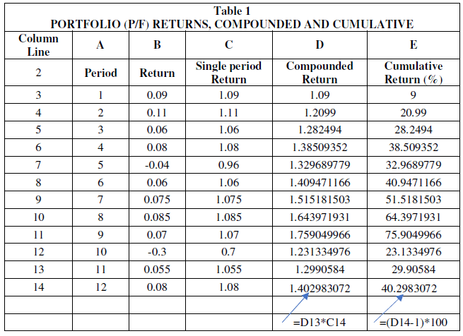

Figure 1 Conceptual framework
From Table 1 we observe that the portfolio has a cumulative return over the 12 periods 40.3% approximately.
However, it should be noted that this yield only makes sense if the returns of the portfolio are reinvested and earn interest over time.
One of the objectives of the portfolio manager is to add value to the managed capital more than the performance of a benchmark such as the stock market index. Suppose that over the 12 time periods benchmark returns are as in column B in Table 2. We thus calculate the Geometric Added Value (GAV):
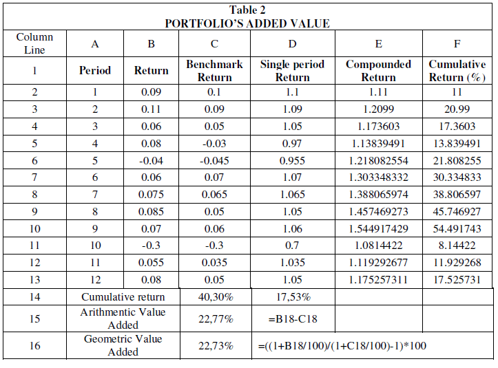
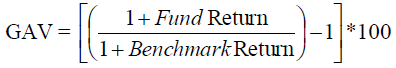 (1)
(1)
Risk Measures
The most important characteristic of the distribution of returns in a portfolio is its risk. Asset allocation decisions have the greatest impact on the risk a portfolio will face. Being able to quantify the risk of a portfolio allows investors to optimize potential returns because the better risk management, the more capital can be allocated to riskier assets that generate the highest returns.
Absolute Risk Measures
The usual measure of the volatility of a returns series is the variance and its standard deviation, which equals the square root of variance. Note that the unit of measurement for the variance is the square of the original unit while its standard deviation restores the original units of measurement (here %). Mean Absolute Deviation (MAD) is the sum of the absolute difference of returns from the average return divide by the number of time periods in Figure 2.

Figure 2 Conceptual framework
Value-at-Risk (VaR) is used to quantify risk and applies to any financial instrument. VaR measures the potential loss in value of a risky asset or portfolio over a defined period for a given confidence interval. Regulators also have become interested in the measure of VaR (Basel Committee on Banking Supervision, SEC and almost all regulatory authorities). According to Jorion (2006) “VaR describes the quantile of the projected distribution of gains and losses over the target horizon. Intuitively, VaR summaries the worst loss over a target horizon with a given level of confidence. VaR is measured in currency units, which makes it more intuitive to understand. VaR is also based on the current positions, so is a forwardlooking measure of risk”
The simple VaR calculation is given in Figure 3. In its simple calculation VaR is computed as:

Figure 3 Conceptual framework
 (2)
(2)
Where α is the confidence level and SD the standard deviation of the portfolio returns. For a more detailed discussion on the advantages and disadvantages of the various techniques estimating VaR and the Monte Carlo simulation method according to the Basel Committee regulatory framework refer to Kalyvas et al (2004). In our case we find that the portfolio worth USD 200,000 cannot have an expected loss of more than USD 42,300.5 per month at 95% of the time. In contrast, the VaR for the benchmark is USD 37,400 approximately per month.
Investors are aware about downside losses versus upside gains. That is investors associate risk with negative returns or, more generally, returns below their expectations. The history of downside risk measures is long, and several such risk measures have been suggested in the literature (Nawrocki 2005), for a brief history of the downside risk measures and Estrada (2006). Example: consider the case where between two portfolios one has a risk of 4.13% and the other 0.35%. The average return of the first is 33.87% and of the second –75.25%. With only the criterion of a standard deviation of returns, a conservative investor would probably choose the second investment. Therefore, the criterion of standard deviation alone is not enough.
The first risk measure in the category of the downside risk measures is semi-variance and its associated semi-deviation:
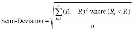 (3)
(3)
The semi-variance is like the variance except that in the calculation no consideration is given to returns above the expected return. That is, it measures downside volatility or, more precisely, volatility below the average return. Instead of the average return one could put the benchmark return, the risk-free rate or any other value. Similarly, other risk measures in the same category include:
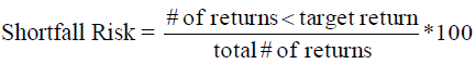
(i). Shortfall Risk:
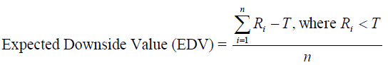
(ii). Expected Downside Value:
 (4)
(4)
where Τ is the target-return.
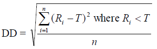
(iii). Downside Deviation:
 (5)
(5)
From Table 3 we see that:
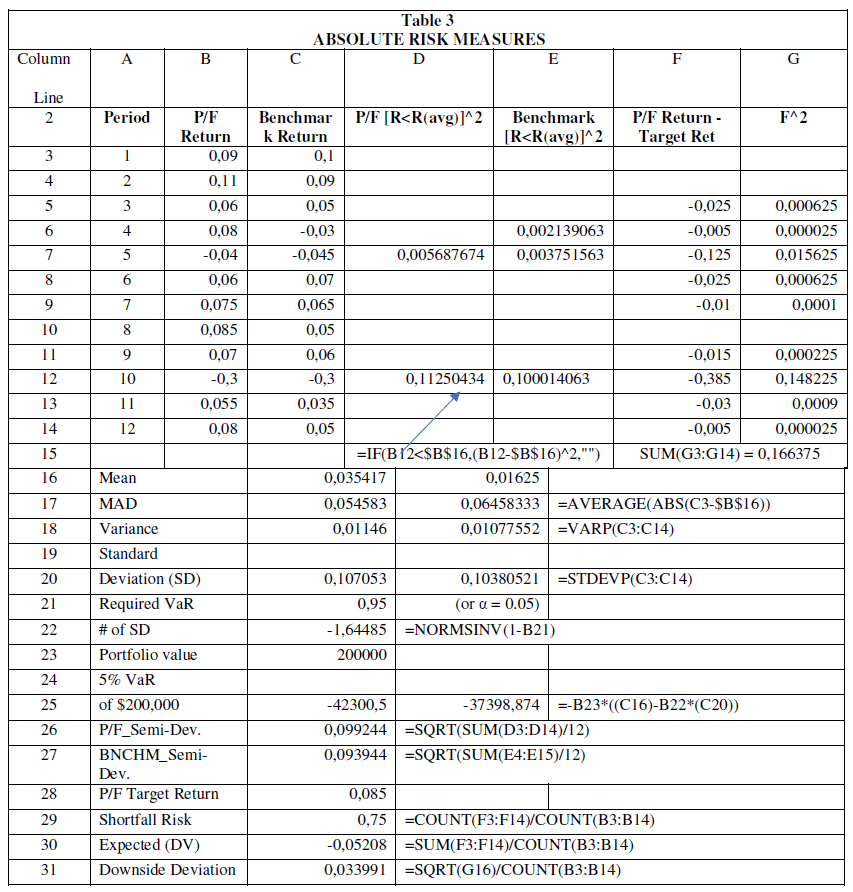
(i). The semi-variance, i.e. the volatility of the portfolio returns that are less than the average return is equal to 9.924%, compared to the standard deviation of 10.7%.
(ii). The shortfall risk size was found to be 75% when the target return was set at 8.5%. That is, 75% of periodic returns are less than 8.5% per month.
(iii). The expected maximum loss (EDV) was found to be -5.2%, given the target yield of 8.5%. That is, when returns fall below the target return, they fall by an average of 5.2% per month.
(iv) The downside deviation (DD) was found to be 3.34%.
Relative Risk Measures
One of the goals of portfolio management is to add value to a benchmark. The benchmark is selected to guide the desired level of risk that the investment strategy wants to take. If the benchmark is chosen in such a way that on the one hand it reflects the aversion to the investor's risk and, on the other hand it gives the expected target return of the investor, then what ultimately counts is to assess the portfolio risk in relation to the risk of the benchmark. If the portfolio was riskier than the benchmark, then the rational investor expects higher returns. On the other hand, if the risk of the managed portfolio is less than that of the benchmark, then the manager probably avoided taking risks that would give him higher returns and therefore did not meet the long-term goals of his/her customer in Table 3.
Thus, while the standard deviation is a satisfactory approximation of the absolute magnitude of the risk of portfolio returns, the relative risk is calculated from how portfolio returns, and benchmark returns change over time.
If the returns on the portfolio and the benchmark are moving up and down at the same time, then there is a degree of absolute risk measured by the standard deviation, but there is no relative risk. If, on the other hand, the returns of the portfolio and the benchmark are not synchronized, for example, if the returns of the portfolio are more negative than the returns of the benchmark in downward markets, then the portfolio has a greater relative risk than the benchmark. Therefore, either the investment strategy needs to be reviewed or the manager's ability needs to be tested or both.
The first two of these quantities is the covariance coefficient (cov) and the correlation coefficient (ρ) of benchmark (B) returns and the portfolio returns (P) respectively:
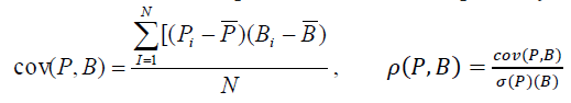 (6)
(6)
where, N is the number of periods,  is the standard deviation of portfolio returns, and
  is the standard deviation of benchmark returns. The correlation coefficient range is from
-1 to +1. If the value of the correlation coefficient is equal to +1, then the returns of the two
quantities are perfectly positively correlated with each other, while if it is equal to -1, then
their returns are perfectly correlated negatively with each other. In case it gets the value zero,
then the returns of the portfolio and the benchmark are unrelated to each other.
is the standard deviation of benchmark returns. The correlation coefficient range is from
-1 to +1. If the value of the correlation coefficient is equal to +1, then the returns of the two
quantities are perfectly positively correlated with each other, while if it is equal to -1, then
their returns are perfectly correlated negatively with each other. In case it gets the value zero,
then the returns of the portfolio and the benchmark are unrelated to each other.
When the portfolio returns and the benchmark returns are simultaneously either higher or lower than their average return, then the covariance takes a high value. The opposite happens when their odds are moving in the opposite direction. When the value of the covariance is very close to zero (or zero), then this is an indication that the choice of the benchmark is not appropriate for the needs of the portfolio.
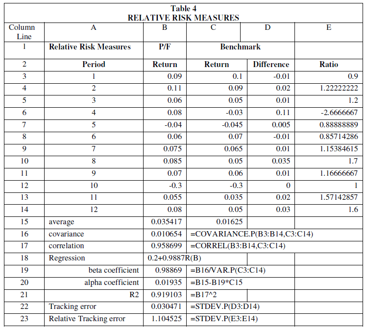
The square of the correlation coefficient gives us the coefficient of determination, R2. The coefficient of determination measures that part of the portfolio returns volatility that is interpreted by the benchmark returns volatility in our example. The range of values of the coefficient of determination is between 0 and 1, incl. When the value of the coefficient of determination R2 approaches the unit, then the volatility of the portfolio returns is significantly interpreted by the volatility of the benchmark returns. In our example it is (0.9586)2 = 0.9191, approximately. That is, the interpretability of the volatility of portfolio returns from the volatility of benchmark returns is very high.
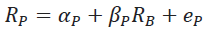
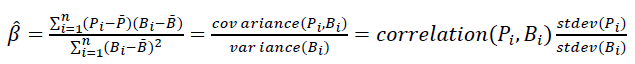
The beta coefficient (or systematic risk) measures the degree to which portfolio returns change, given the volatility of benchmark returns. The beta isolates the degree of market risk (benchmark) inherent in the portfolio, where the risk is determined by the overall volatility of returns. A very high beta value indicates that the portfolio has a higher risk than the benchmark. If the beta value is less than 1, then the portfolio returns are less volatile than the benchmark returns. If the beta value is higher than the unit, then the portfolio returns have a higher volatility, in terms of their average return over the study period, relative to those of the benchmark. Finally, a value of beta close to zero means that there is little correlation between portfolio returns and benchmark. The beta coefficient is the slope of the regression:
 (7)
(7)
Where  is the beta coefficient,
  is the intercept term,
  and
and  the portfolio and
benchmark returns respectively, and
the portfolio and
benchmark returns respectively, and  represents the random factor. The estimation of beta
factor is then given by:
represents the random factor. The estimation of beta
factor is then given by:
 (8)
(8)
A negative value of the covariance between P and B will lead to a negative beta value (the standard deviation can never be negative), which means that there is an inverse relationship between the portfolio returns and the benchmark returns. The intercept term (known Jensen’s α measure) as is estimated be:
 represents the average return of the portfolio and the
benchmark respectively. Hence, the estimated regression is: 0.02+0.9887R(B) with coefficient
of determination R2 = 0.9191
represents the average return of the portfolio and the
benchmark respectively. Hence, the estimated regression is: 0.02+0.9887R(B) with coefficient
of determination R2 = 0.9191
From the results, beta coefficient of the portfolio is equal to about 0.9887 and is less than one. The alpha coefficient (or Jensen’s α. In fact, Jensen’s α coefficient is estimated by using CAPM) was found to be equal to 0.02 approximately. This means that the expected portfolio returns on average are equal to the 0.988 time the benchmark’s returns plus 0.2%. Finally, the coefficient of determination is 0.9191, which means that the returns of the portfolio are explained by the returns of the benchmark at 91.91%.
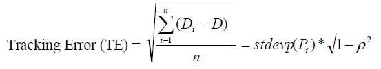
Tracking Error (or active risk) quantifies the differences between portfolio and benchmark returns and is most useful when the administrator follows the benchmark "closely". If the portfolio manager follows exactly the benchmark (i.e. the portfolio is an index fund), then the linear correlation coefficient of the portfolio returns and the benchmark will be equal to one and, at the same time, the value of the tracking error will be equal to zero.
 (9)
(9)
where D is the difference between the portfolio and benchmark’s returns, and ρ is the correlation coefficient between the two series.
The size of tracking error represents the "cost" of active management, in the sense that the variability of portfolio returns from benchmark returns represents the noise that couldn’t be controlled and managed by the portfolio manager and, of course, which has an impact on management performance. Similarly, the relative tracking error value is estimated by:
 (10)
(10)
In our example both the tracking error and the relative tracking error are found very low. Figure 3 summarizes the relative risk measures for our case study in Table 4.
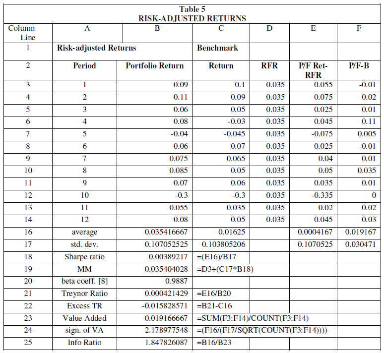
Valuation of absolute returns adjusted to the risk
Usually, a portfolio manager is interested in evaluating his performance in relation to the risk taken. Thus, various risk-adjusted performance measures have been developed, such as the Sharpe index, the Treynor index (1966), the Modigliani and Modigliani index (MM or M2), based on modern portfolio theory and the CAPM. One of these measures is the risk adjusted return (RAR) defined by the ratio of the average return divided by the standard deviation of the returns. RAR is the inverse of the coefficient of variation (CV).
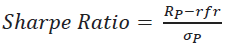
W. Sharpe (1966) introduced a measure for the performance of mutual funds and proposed the term reward-to-variability ratio to describe it and has gained considerable popularity, under various names by different authors such as Sharpe Index, Sharpe Measure, or Sharpe Ratio. The basic idea is that we can no longer achieve a risk-free return without taking a risk (reward-to-variability ratio). Sharpe Ratio measures the performance of an investment (e.g., a security, a portfolio, an index or a mutual fund) compared to a risk-free asset, after adjusting for its risk. It is thus defined as the difference between the returns of the investment and the risk-free return divided by the standard deviation (risk) of the investment (i.e., its volatility). Therefore, it represents the additional amount of return that an investor receives per unit of increase in risk.
 (11)
(11)
where the nominator presents the excess return of the portfolio, rfr is the risk-free rate and  is the standard deviation of the portfolio’s excess return.
Theoretically, the risk-free rate is the rate of return of an investment with zero risk and represents the return an investor would expect from a risk-free investment. It can be estimated as the difference between the current inflation rate from the yield of the Treasury bond matching the desired investment duration. In this case we assume a risk-free rate 3.5%. The higher the value of this index, the higher the return on the portfolio per risk unit.
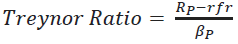
The Treynor ratio, also known as the reward-to-volatility ratio, is a performance metric for determining how much excess return was generated for each unit of risk taken on by a portfolio. Risk in the Treynor ratio refers to systematic risk as measured by a portfolio's beta coefficient and not the risk of the portfolio as in Sharpe Ratio. As we know beta factor measures the tendency of a portfolio's return to change in response to changes in return for the overall market (or the benchmark in our case study). Treynor is calculated as:
 (12)
(12)
where is the systematic risk (beta coefficient) of the portfolio. The higher the value of this
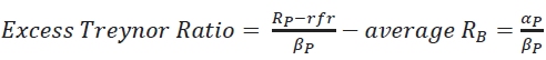
index, the higher the return on the portfolio per risk unit. We also can estimate the Excess
Treynor Ratio that is directly related to abnormal performance. These two measures are
roughly equivalent. Nevertheless, the link between the Excess Treynor ratio and Jensen's alpha is easier to interpret: the Excess Treynor ratio is just the equal to the alpha coefficient
per unit of systematic risk of the portfolio:
 (13)
(13)
where is the intercept of the regression [8] or Jensen’s alpha coefficient.
Review of Previous Studies
The Modigliani and Modigliani index is given by Modigliani and Modigliani (1997):
 (14)
(14)
The MM measure is equivalent to the return the portfolio would have achieved if it had the same risk as the market index or any other benchmark. Again, the higher the value of this index, the higher the return on the portfolio per unit of risk.
The information ratio (or appraisal ratio) measures and compares the active return of an investment compared to a benchmark index relative to the volatility of the active return. It is defined as the ratio of the difference between the returns of the portfolio and the returns of the benchmark divided by the tracking error. It represents the additional amount of return that an investor receives per unit of increase in risk (Clarke et al. 2015):
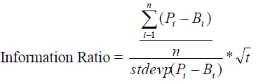 (15)
(15)
Based on what we said about the tracking error, we can consider information ratio (IR) as a "benefit - cost" ratio, which evaluates the ability of the portfolio manager to access information. The portfolio manager with higher IR adds more value to the portfolio per unit deviation from the benchmark. A value of the IR greater than one can be interpreted as an indication of the ability of the manager. A negative value indicates that the manager achieved a performance lower than the benchmark. In practice, IR values between 0.5 and 1.0 are considered satisfactory.
Overall, as it is evident from Table 5, portfolio manager in our case study performed quite well. Based on the calculated t-student statistic (“sign. of VA”) in the added value, one could accept the hypothesis that the portfolio manager's added value is statistically significant, which confirms the previous conclusion (however, it should be noted that this is a simple case study with very few observations).
The Multi-Manager Investment Model
However, we have not yet answered the question: how is the systematic value-added ability of a portfolio manager evaluated? In this case, the runs test, among other things, can help us. Suppose that in addition to our portfolio manager we have two more managers namely, FM1, FM2 and FM3. The question is to compare the stability of their performance over time.
As noted in Mass Mutual Investment (2020) “multi-manager funds have become increasingly popular among 401(k) and other retirement investors in recent years. Fund-offunds (FoF) managers and multi-managers were some of the first institutional real estate practitioners whose days were numbered following the 2008 financial crisis. … This is not surprising since these vehicles can offer several attractive advantages over other investment alternatives particularly for investors focused on better retirement outcomes. However, maximizing these benefits depends on a well-thought out and disciplined process, highlighted by a rigorous approach to manager search and selection, pairing and ongoing monitoring”. Columns B, C, D give the performance of the 3 portfolio managers.
The next three columns with "1" mark if there was added value and with "0" if not. Columns I, J, K indicate if there is a trend in their success for value added or reversal of this trend. The excel COUNT function measures the number of value-added trend pauses. The POSSIBLE function counts the number of minimum possible pauses. Finally, the RUNS command gives the value of the ratio of the two previous ones.
If a portfolio manager systematically adds value to the portfolio, then we expect the smallest number of downtimes. If it accidentally added value to the portfolio, then RUNS = 0.5. If RUNS→0, then the manager adds value systematically (i.e., there is a trend). The opposite if it approaches the unit.
Table 6 clearly shows that FM3 performs better than the other two portfolio managers as expected. In fact, both FM1 and FM2 should be fired.
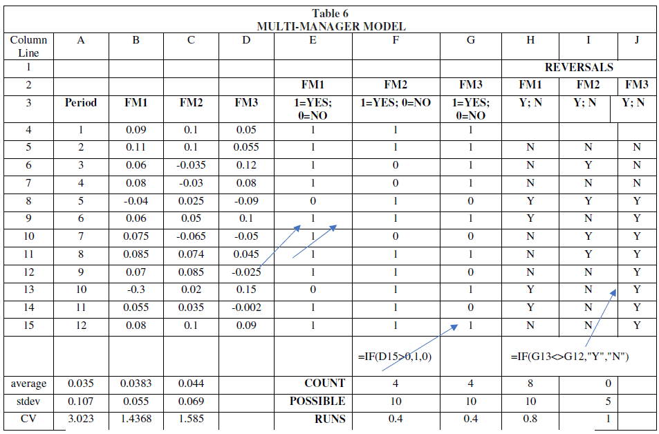
From Figure 3 is evident that FM2 presents the more stable returns over time. FM1 has one very negative return, and FM3 is quite stable with better returns. Thus, we expect that FM3 is more skillful as compared with FM1 and FM2.
Performance Attribution
Performance attribution or investment performance attribution is a set of techniques used to compare portfolio’s performance with benchmark’s performance and identify the added value of the portfolio’s active management. Attribution analysis compares the total return of the manager's actual investment holdings with the return for a predetermined benchmark portfolio and decomposes the difference into a selection effect and an allocation effect. The objective of this analysis is to distinguish which of the two factors of portfolio performance, superior asset selection or superior market timing, is the source of the portfolio's overall performance (Bacon 2019).
I will close the presentation of portfolio performance analysis with two key options:
(j) the allocation effect; and
(ii) the selection of the individual assets (selectivity effect) of the portfolio.
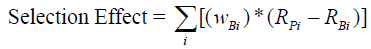
The overall performance of a portfolio can be decomposed into measures of risk-taking and security selection skill. The purpose of this analysis is to determine the effect of value added on the portfolio from these manager options. The relationships used are:

 (16 a, b)
Where, wPi are the weights in the portfolio followed by the manager for each asset i (stock, industry, etc.) and wBi are the corresponding weightings of item i in the benchmark. RPi and RBi are the respective odds and RB is the overall performance of the benchmark. In this way the result of the allocation evaluates the manager's choice to over- under- value a specific asset or industry [i.e.,(wPi - wBi)] on the variation of the returns of this asset in relation to the overall return of the benchmark [i.e.,( RBi - RB)].
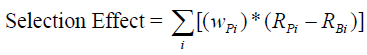
The ability of the manager to synchronize with the market refers to the manager's choice to invest most of the managed capital in the asset that will give the highest return. The result of the selection evaluates the ability of the manager to structure segments (or even individual shares, for example) in the portfolio, which result in a higher return than that of the corresponding segment in the benchmark [i.e., , (RPi - RBi )] weighted appropriately by the manager [ that is, ( wPi)]. Thus, the total added value of the administrator is derived from the sum of these two components.
Alternatively, the selection effect can be calculated as:
 (17)
(17)
where, the weighting is that of the benchmark. But because in this way the sum of the distribution result and the selection result does not add up to the total result, the interaction effect is calculated to evaluate the residual effect as:
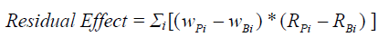 (18)
(18)
In the example of Table 7, the way of calculating the two results, distribution and selection is presented. In this example, the manager achieved better performance than the benchmark.
The total return on the portfolio (the sum of the products of the weightings on the returns on the assets of the portfolio) was 8.98% compared to the corresponding total return on the market index portfolio, which was equal to 8.46%. The difference achieved by the πορτφολιο μαναγερ was 52 basis points (= 0.0898 -0.0846). This added value is broken down into the allocation result and the selection effect.
The allocation effect was found to be -0.016%, which is divided into -0.014% (or -1.4 basis points) of shares, 0.06% (or 6 basis points) of bonds and -0.06% (or -6 basis points) from holding cash. The manager, overall, achieved better performance than the market index portfolio, but had a negative allocation effect. This means that it had a positive selection effect. The selection result by alternative method (17) was found to be equal to 0.65%, while by calculation method (16 a&b) was found to be equal to 0.53%. The residual result was -0.11%. Therefore, the total value added in the portfolio was equal to 0.52% (or 52 basis points), broken down into either [0.634 -0.114)] or [0.536 + (-0.016)].
Conclusion
In this short note a comprehensive analysis of the performance of a portfolio along with manager’s ability to offer additional value is presented. The study followed CFA methodology and all calculations are made in excel using simple formulas. This is the first step in understanding portfolio evaluation. I also advise the students to refer to the textbooks listed in “Further Reading”.
Advanced inquiries on portfolio attribution and managers evaluation include questions such as the “hot hands” phenomenon and the style analysis of fund managers Papadamou & Siriopoulos (2004) or the multi-factor analysis, which attributes performance to factors such as economic variables, fundamental variables, technical analysis factors etc., or the performance of alternative investments, especially in periods where interest rates and returns in traditional investment vehicles are relatively low Baker & Filbeck (2013).
Further Reading
Evaluating an investment portfolio is a complex and detailed process that encompasses a great deal more than analyzing investment returns. This section contains a list of textbooks, which a reader may consult for additional and more detailed coverage on portfolio performance.
1). Frank K. Reilly and Keith C. Brown (2012). Investment Analysis & Portfolio Management, Tenth Edition, South-Western, Cengage Learning. Pages 1045.
Especially Part 7, Chapter 24 and Chapter 25.
Level of difficulty: Intermediate.
2). Edwin J. Elton, Martin J. Gruber, Stephen J. Brown, and William N. Goetzmann (2014). Modern Portfolio Theory and Investment Analysis, 9th edition, Wiley. Pages 731.
Especially Part 5, Chapters 25-28.
Level of difficulty: Advanced.
3). Bodie, Kane, and Marcus (2020). Investments, McGraw Hill, 11th edition.
Especially Part VII, Chapters 24-28.
Level of difficulty: Easy.
References
- Aragon, O.G., & W.E. Ferson (2006). Portfolio Performance Evaluation, Foundations and Trends in Finance, 2(2), pp. 83-190. DOI: 10.1561/0500000015
- Aven, T. (2016). Risk assessment and risk management: Review of recent advances on their foundation, European Journal of Operations Research, 253(1), pp. 1-13. http://dx.doi.org/10.1016/j.ejor.2015.12.023
- Bacon, Carl R. (2019). Performance Attribution History and Progress. CFA Institute Research Foundation. p. 42.
- Baker, H.K., & Filbeck G., (2013). Alternative Investments: Instruments, Performance, Benchmarks, and Strategies. Wiley.
- Benninga, S. (2014). Financial Modeling. 4th edition, MIT Press.
- Bodie Z.,A. Kane, & A.J. Marcus (2014). Investments. 10th edition. New York (US): McGraw-Hill Education.
- Clare, A. Performance Evaluation, CFA Institute, Chapter 19.
- https://www.cfainstitute.org/-/media/documents/support/programs/investment-foundations/19-performance-evaluation.ashx?la=en&hash=F7FF3085AAFADE241B73403142AAE0BB1250B311
- Clarke, Roger G., de Silva, Harindra, & T. Steven (2015), Analysis of Active Portfolio Management, CFA Institute.
- Elton, J.E., M.A. Gruber (1995). Modern portfolio theory and investment analysis, 5th Edition. Toronto: John Wiley and sons.
- Estrada, J. (2006). Downside Risk in Practice. Journal of Applied Corporate Finance, 18(1), pp. 117-125.
- Fabozzi, J. F., & J.L. Grant (2001). Equity Portfolio Management, Wiley.
- Gkillas, K.C. Konstantatos, A. Tsagkanos, & C. Siriopoulos (2020), “Do economic news releases affect tail risk? Evidence from an emerging market”, Finance Research Letters, August 2020 https://www.sciencedirect.com/science/article/abs/pii/S154461232030297X
- IOSCO (1998). Risk management and control guidance for securities firms and their supervisors, A Report by the Technical Committee of the International Organization of Securities Commissions, May. https://www.iosco.org/library/pubdocs/pdf/IOSCOPD78.pdf
- Jones, C.P. (2009). Investments: Analysis and Management (11th ed.), New Jersey: John Wiley & Sons.
- Jorion, P. (2006). Value at Risk. Mac Graw-Hill.
- Kalyvas, L., Dritsakis, N., Siriopoulos, C. et al. Selecting Value-at-Risk methods according to their hidden characteristics. Operations Research an International Journal, 4(167) https://doi.org/10.1007/BF02943608
- Mass Mutual Investment (2020). The Multi-Manager Approach.
- https://www.massmutual.com/mmfunds/The-Multi-manager-Approach-A-Better-Fit-for-Retirement-Investors.pdf
- Modigliani, F., & J. Modigliani (1997). Risk-adjusted performance, Journal of Portfolio Management, 23(2), pp. 45-54
- Nawrocki, D. (2005). A Brief History of Downside Risk Measures. Journal of Investing, 8(3). DOI: 10.3905/joi.1999.319365
- Markowitz H. (1952). Portfolio selection, The Journal of Finance, 7(1), pp. 77-91.
- Papadamou, S., & C. Siriopoulos (2004). American equity mutual funds in European markets: Hot hands phenomenon and style analysis, International Journal of Finance and Economics, 9, p.p. 85-97.
- Reilly, F., K. Brown, & S. Leeds (2018). Investment Analysis and Portfolio Management, 11th edition, Cengage Learning, Inc
- Sharpe, William F. "Mutual Fund Performance." Journal of Business, January 1966, pp. 119-138.
- Treynor, Jack L. (1966). “How to rate management investment funds.” Harvard Business Review, 43(1), pp. 63-75.