Case Reports: 2018 Vol: 24 Issue: 3
Sensitivity Analysis in Linear Programing: Some Cases and Lecture Notes
Samih Antoine Azar, Haigazian University
Case Description
This paper presents case studies and lecture notes on a specific constituent of linear programming, and which is the part relating to sensitivity analysis, and, particularly, the 100% rule of simultaneous changes or perturbations. First, proportional perturbations in the coefficients of the objective function are studied. Then, proportional perturbations on the right-hand side coefficients of the constraints are effectuated. Moreover, the paper starts from a limitation of the 100% rule for simultaneous perturbations. This classic 100% rule applies only to perturbations in opposite direction. The paper proposes a modified 100% rule that can accommodate perturbations in the same direction, and that seems to work well in most circumstances. The simulations include 4-variable and 3-variable linear programs, and covers both maximization cases and minimization cases. It is hoped that these simulations will make this part of sensitivity analysis more amenable to students, and that it will provide animated and lively discussions in the class room. Likewise, it is expected that teachers, academicians, and professionals will benefit from the various suggested insights in this paper.
Case Synopsis
Linear programming models have a privileged place in operations research and management science. These models apply to more than one field in business, economics, and in the social sciences. Originally, the thrust of the research was directed to the complexity of the simplex method for reaching the optimal solution (Dorfman et al., 1958, reprinted 1986). However, with the advent of optimization and numerical techniques, and with advances in computer memory and speed, the simplex method was relegated to being just a curiosity. A linear program consists in a linear value function to be optimized (maximized or minimized) and a set of linear constraints that must be satisfied. In case of maximization of the total contribution margin, which is the benchmark example, these constraints can be equalities or inequalities. They are usually referred to as capacity constraints, or resource constraints. The presence of such constraints makes the linear program essentially of a short run nature, because in the long run resources are quasi unlimited. But this is not always necessary. For a variety of applications of linear programs the reader is referred to Anderson et al. (2016).
The celebrity of linear programming is not only due because it provides diligently for solutions to problems but because it provides also for sensitivity analysis. Sensitivity measures how robust the optimal solution is. It applies to changes in the coefficients of the objective function value or to changes in the right-hand side values of the constraints. These changes can be either on one parameter only or simultaneously on more than one parameter. It is especially appropriate whenever there is uncertainty in estimating with precision the magnitude of some or all the parameters in the program. There are many approaches to sensitivity analysis. Ward and Wendell (1990) is a topical review. In this paper we are concerned with what has been called the 100% rule by its originators (Bradley et al., 1977). This rule consists of summing up the relative values of the actual change in a coefficient over the maximum allowable change of that same coefficient (upper or lower limit). See Filippi (2011) and Anderson et al. (2016). Filippi (2011) is a recent derivation of the 100% rule, and he states that “if we are interested in perturbations that increase the right-hand side coefficients, we need to check only one (additive) inequality”. As an instance if the current value of a coefficient is 20 and the maximum allowable decrease, or lower limit, is 10, then a change to 15 corresponds to the following ratio:
(15-20)/(10-20)=0.50
If another coefficient has a current value of 12 and a maximum allowable change or upper limit of 25, then a change to 16 corresponds to the following ratio:
(16-12)/(25-12)=0.31
Summing up these two ratios produces:
0.50+0.31=0.81<1=100%
And the 100% rule is satisfied. The rule is not satisfied if the sum falls above 1 or 100%.
What conclusions can we draw in this case? If the two changes are for coefficients of the objective value function, then:
1. The optimal solution does not change.
2. The total value of the objective function changes.
3. Knowing the changes in the coefficients, the new level of the objective function can be calculated.
If the two changes are for the right-hand side parameters of the constraints of the problem, then:
1. The dual or shadow prices do not change.
2. The solution changes.
3. The binding constraints remain binding.
4. The non-binding constraints remain non-binding.
5. The total value of the objective function changes.
6. Knowing the intended changes, and knowing the dual prices, one can calculate the change in the value of the objective function, and from there the total of the new function value. For each constraint the change in the constraint parameter is multiplied by the dual price of that constraint and then appropriately summed up across the two constraints.
These outcomes are said to be a part of a sensitivity analysis in the linear program. Briefly checking whether the 100% rule is satisfied and adopting the implied results is the purpose of sensitivity analysis.
If the program is composed of only two decision variables, then there is a second method for obtaining the new value of the objective function. This is by solving first for the new optimal solution from the binding constraints, and replacing this solution in the objective function.
In case the 100% rule is not satisfied we conclude that we need to resolve the problem. The optimal solution may not change if the changes are in the coefficients of the objective function. And the shadow prices may not change if the changes are in the right-hand side parameters. Therefore, in this case, there is ambiguity and we are not sure about what will happen. Satisfying the 100% rule has strong implication on either the solution, or the dual prices. But if the 100% rule is not satisfied then one cannot say that either the solution changes or that the dual prices change, but simply: we need to resolve. The solution and the dual prices may not change despite the rejection of 100% rule.
There is a caveat. The 100% rule described above applies only for changes in opposite direction although this is not clear from the textbook that reports it (Anderson et al., 2016). For changes in the same direction the 100% rule must be modified. This paper will propose a modification of the 100% rule later which works well in most circumstances. Simply put, the new rule is by taking the absolute value of the subtraction of the percent relative changes. The fundamental change in the rule is subtraction instead of addition, while taking absolute values.
This paper is organized as follows. In the following section, section 2, the two case-problems that will be studied are presented, together with the reason for their selection. In this section, the different scenarios are also depicted. Section 3 dwells upon the cases where the objective functions are multiplied threefold. Section 4 dwells upon the cases when the coefficients of the right-hand side constraints are multiplied threefold. Section 5 dwells upon simultaneous perturbations in the right-hand side coefficients of the constraints. Section 6 dwells upon simultaneous perturbations in the coefficients of the objective functions. The final section summarizes and concludes. In sections 5 and 6 is introduced the modified 100% rule for simultaneous perturbations in the same direction. This rule seems to work well in most circumstances, and, hence, should be included in more recent editions of textbooks on operations research.
Linear Program Setup
At first, two linear programs will be studied, one maximization and one minimization. The maximization will consist of three or four decision variables. This choice is made for the purpose of illustrating higher-order problems. Likewise, the minimization will consist of three or four decision variables. The purpose is to be as general as possible. Each linear program will be subjected to two perturbations, one by multiplying the objective function by three, keeping the same constraints, and the other by multiplying the right-hand side values by three, keeping the same objective function. The scalar 3 is arbitrary. The impact of these perturbations on the initial solution will be analyzed and reported.
For the maximization with 4 decision variables, two different perturbations will be applied. Both are carried out by choosing arbitrarily the perturbations. These perturbations will be effectuated on the right-hand side coefficients of the constraints. The modified 100% rule will be restated and solved. The purpose is the selection of perturbations that lead to failure of the ordinary 100% rule. For the minimization with four decision variables the two independent and arbitrary perturbations are imposed on the right-hand side coefficients of the constraints and they are selected in such a way as to have them fail the ordinary 100% rule. The results of all these perturbations will be analyzed and classified.
The maximization with four decision variables is as follows:
Maximize: X1+X2+2X3+2X4
Subject to:
X1+2X2+3X3+3X4 ≤ 15,000
2X1+4X2+X3+3X4 ≤ 20,000
3X1+2X2+5X3+3X4 ≤ 20,000
X1 ≥ 1,000
X2 ≥ 1,000
X3 ≥ 1,000
X4 ≥ 1,000
The non-negativity constraints will apply always but are not listed and repeated. The solution and sensitivity analysis to this linear program are presented in Table 1. The computer output has been processed using the Management Scientist® software, a copy of which is appended to the textbooks of Anderson et al. (2016).
| Table 1 MAXIMIZATION OF THE 4-VARIABLE LINEAR PROGRAM: BASIC SOLUTION |
||||||
| OPTIMAL SOLUTION | ||||||
| Objective Function Value=10166.667 | ||||||
| Variable | Value | Reduced Costs | ||||
| X1 | 1500.000 | 0.000 | ||||
| X2 | 1000.000 | 0.000 | ||||
| X3 | 1000.000 | 0.000 | ||||
| X4 | 2833.333 | 0.000 | ||||
| Constraint | Slack/Surplus | Dual Prices | ||||
| 1 | 0.000 | 0.500 | ||||
| 2 | 3500.000 | 0.000 | ||||
| 3 | 0.000 | 0.167 | ||||
| 4 | 500.000 | 0.000 | ||||
| 5 | 0.000 | -0.333 | ||||
| 6 | 0.000 | -0.333 | ||||
| 7 | 1833.333 | 0.000 | ||||
| OBJECTIVE COEFFICIENT RANGES | ||||||
| Variable | Lower Limit | Current Value | Upper Limit | |||
| X1 | 0.667 | 1.000 | 2.000 | |||
| X2 | No Lower Limit | 1.000 | 1.333 | |||
| X3 | No Lower Limit | 2.000 | 2.333 | |||
| X4 | 1.500 | 2.000 | 3.000 | |||
| RIGHT HAND SIDE RANGES | ||||||
| Constraint | Lower Limit | Current Value | Upper Limit | |||
| 1 | 11333.333 | 15000.000 | 16000.000 | |||
| 2 | 16500.000 | 20000.000 | No Upper Limit | |||
| 3 | 19000.000 | 20000.000 | 27000.000 | |||
| 4 | No Lower Limit | 1000.000 | 1500.000 | |||
| 5 | 0.000 | 1000.000 | 2750.000 | |||
| 6 | 0.000 | 1000.000 | 1500.000 | |||
| 7 | No Lower Limit | 1000.000 | 2833.333 | |||
The minimization with four decision variables is as follows:
Minimize: 0.4X1+0.2X2+0.2X3+0.3X4
Subject to:
X1+X2+X3+X4 ≥ 36
3X1+4X2+8X3+6X4 ≥ 280
5X1+3X2+6X3+6X4 ≥ 200
10X1+25X2+20X3+40X4 ≥ 280
The solution and the sensitivity analysis of this linear program are presented in Table 2.
| Table 2 MINIMIZATION OF THE 4-VARIABLE LINEAR PROGRAM: BASIC SOLUTION |
||||||
| OPTIMAL SOLUTION | ||||||
| Objective Function Value=7.200 | ||||||
| Variable | Value | Reduced Costs | ||||
| X1 | 0.000 | 0.200 | ||||
| X2 | 2.000 | 0.000 | ||||
| X3 | 34.000 | 0.000 | ||||
| X4 | 0.000 | 0.100 | ||||
| Constraint | Slack/Surplus | Dual Prices | ||||
| 1 | 0.000 | -0.200 | ||||
| 2 | 0.000 | 0.000 | ||||
| 3 | 10.000 | 0.000 | ||||
| 4 | 450.000 | 0.000 | ||||
| OBJECTIVE COEFFICIENT RANGES | ||||||
| Variable | Lower Limit | Current Value | Upper Limit | |||
| X1 | 0.200 | 0.400 | No Upper Limit | |||
| X2 | 0.100 | 0.200 | 0.200 | |||
| X3 | 0.200 | 00.200 | 0.400 | |||
| X4 | 0.200 | 0.300 | No Upper Limit | |||
| RIGHT HAND SIDE RANGES | ||||||
| Constraint | Lower Limit | Current Value | Upper Limit | |||
| 1 | 35.000 | 36.000 | 70.000 | |||
| 2 | 266.667 | 280.000 | 288.000 | |||
| 3 | No Lower Limit | 200.000 | 210.000 | |||
| 4 | No Lower Limit | 280.000 | 730.000 | |||
Multiplying Threefold the Objective Functions
The computer outputs relevant to multiplying threefold the objective function are presented respectively in Tables 3 and 4.
| Table 3 MAXIMIZATION OF THE 4-VARIABLE LINEAR PROGRAM: THE OBJECTIVE FUNCTION MULTIPLIED THREEFOLD |
||||||
| OPTIMAL SOLUTION | ||||||
| Objective Function Value=30500.000 | ||||||
| Variable | Value | Reduced Costs | ||||
| X1 | 1500.000 | 0.000 | ||||
| X2 | 1000.000 | 0.000 | ||||
| X3 | 1000.000 | 0.000 | ||||
| X4 | 2833.333 | 0.000 | ||||
| Constraint | Slack/Surplus | Dual Prices | ||||
| 1 | 0.000 | 1.500 | ||||
| 2 | 3500.000 | 0.000 | ||||
| 3 | 0.000 | -0.500 | ||||
| 4 | 500.000 | 0.500 | ||||
| 5 | 0.000 | -1.000 | ||||
| 6 | 0.000 | -1.000 | ||||
| 7 | 1833.333 | 0.000 | ||||
| OBJECTIVE COEFFICIENT RANGES | ||||||
| Variable | Lower Limit | Current Value | Upper Limit | |||
| X1 | 2.000 | 3.000 | 6.000 | |||
| X2 | No Lower Limit | 3.000 | 4.000 | |||
| X3 | No Lower Limit | 6.000 | 7.000 | |||
| X4 | 4.500 | 6.000 | 9.000 | |||
| RIGHT HAND SIDE RANGES | ||||||
| Constraint | Lower Limit | Current Value | Upper Limit | |||
| 1 | 11333.333 | 15000.000 | 16000.000 | |||
| 2 | 16500.000 | 20000.000 | No Upper Limit | |||
| 3 | 19000.000 | 20000.000 | 27000.000 | |||
| 4 | No Lower Limit | 1000.000 | 1500.000 | |||
| 5 | 0.000 | 1000.000 | 2750.000 | |||
| 6 | 0.000 | 1000.000 | 1500.000 | |||
| 7 | No Lower Limit | 1000.000 | 2833.333 | |||
| Table 4 MINIMIZATION OF THE 4-VARIABLE LINEAR PROGRAM: OBJECTIVE FUNCTION MULTIPLIED THREEFOLD |
||||||
| OPTIMAL SOLUTION | ||||||
| Objective Function Value=21.600 | ||||||
| Variable | Value | Reduced Costs | ||||
| X1 | 0.000 | 0.600 | ||||
| X2 | 2.000 | 0.000 | ||||
| X3 | 34.000 | 0.000 | ||||
| X4 | 0.000 | 0.300 | ||||
| Constraint | Slack/Surplus | Dual Prices | ||||
| 1 | 0.000 | -0.600 | ||||
| 2 | 0.000 | 0.000 | ||||
| 3 | 10.000 | 0.000 | ||||
| 4 | 450.000 | 0.000 | ||||
| OBJECTIVE COEFFICIENT RANGES | ||||||
| Variable | Lower Limit | Current Value | Upper Limit | |||
| X1 | 0.600 | 1.200 | No Upper Limit | |||
| X2 | 0.300 | 0.600 | 0.600 | |||
| X3 | 0.600 | 0.600 | 1.200 | |||
| X4 | 0.600 | 0.900 | No Upper Limit | |||
| RIGHT HAND SIDE RANGES | ||||||
| Constraint | Lower Limit | Current Value | Upper Limit | |||
| 1 | 35.000 | 36.000 | 70.000 | |||
| 2 | 266.667 | 280.000 | 288.000 | |||
| 3 | No Lower Limit | 200.000 | 210.000 | |||
| 4 | No Lower Limit | 280.000 | 730.000 | |||
For the maximization (Table 3), the results of this multiplication are as follows:
1. The objective function value is multiplied threefold.
2. The optimal solution is the same.
3. The ranges of optimality, i.e. the ranges for the coefficients of the objective function, are multiplied threefold.
4. The dual prices are multiplied threefold.
5. The slack and surpluses remain the same.
6. The binding constraints remain binding.
7. The non-binding constraints remain non-binding.
8. The ranges of feasibility, i.e. the ranges for the right-hand side coefficients, are all the same.
For the minimization (Table 4), the results of this multiplication are as follows:
1. The objective function value is multiplied threefold.
2. The optimal solution is the same.
3. The reduced costs are multiplied threefold.
4. The ranges of optimality, i.e. the ranges for the coefficients of the objective function, are multiplied threefold.
5. The dual prices are multiplied threefold.
6. The slack and surpluses remain the same.
7. The binding constraints remain binding.
8. The non-binding constraints remain non-binding.
9. The ranges of feasibility, i.e. the ranges for the right-hand side coefficients, are all the same.
Multiplying Threefold the Right-Hand Side Coefficients
The computer outputs relevant to multiplying threefold the right-hand side coefficients of the four-variable maximization program are presented in Table 5. For this maximization the results of this multiplication are as follows:
Table 5 MAXIMIZATION OF THE 4-VARIABLE LINEAR PROGRAM: THE RIGHT-HAND SIDE COEFFICIENTS OF THE CONSTRAINTS MULTIPLIED THREEFOLD |
||||||
| OPTIMAL SOLUTION | ||||||
| Objective Function Value=30500.000 | ||||||
| Variable | Value | Reduced Costs | ||||
| X1 | 4500.000 | 0.000 | ||||
| X2 | 3000.000 | 0.000 | ||||
| X3 | 3000.000 | 0.000 | ||||
| X4 | 8500.000 | 0.000 | ||||
| Constraint | Slack/Surplus | Dual Prices | ||||
| 1 | 0.000 | 0.500 | ||||
| 2 | 10500.000 | 0.000 | ||||
| 3 | 0.000 | 0.167 | ||||
| 4 | 1500.000 | 0.000 | ||||
| 5 | 0.000 | -0.333 | ||||
| 6 | 0.000 | -0.333 | ||||
| 7 | 5500.000 | 0.000 | ||||
| OBJECTIVE COEFFICIENT RANGES | ||||||
| Variable | Lower Limit | Current Value | Upper Limit | |||
| X1 | 0.667 | 1.000 | 2.000 | |||
| X2 | No Lower Limit | 1.000 | 1.333 | |||
| X3 | No Lower Limit | 2.000 | 2.333 | |||
| X4 | 1.500 | 2.000 | 3.000 | |||
| RIGHT HAND SIDE RANGES | ||||||
| Constraint | Lower Limit | Current Value | Upper Limit | |||
| 1 | 34000.000 | 45000.000 | 48000.000 | |||
| 2 | 49500.000 | 60000.000 | No Upper Limit | |||
| 3 | 57000.000 | 60000.000 | 81000.000 | |||
| 4 | No Lower Limit | 3000.000 | 4500.000 | |||
| 5 | 0.000 | 3000.000 | 8250.000 | |||
| 6 | 0.000 | 3000.000 | 4500.000 | |||
| 7 | No Lower Limit | 3000.000 | 8500.000 | |||
1. The objective function value is multiplied threefold.
2. The optimal solution is multiplied threefold.
3. The ranges of optimality are the same.
4. The dual prices remain the same.
5. The slacks are multiplied threefold.
6. The binding constraints remain binding.
7. The non-binding constraints remain non-binding.
8. The ranges of feasibility are multiplied threefold.
For the four-variable minimization, the results of this multiplication are the same as above, in the case of the maximization, and will not be repeated.
Simultaneous Perturbations in the Right-Hand Side Coefficients of the Constraints, and the Modified 100% Rule
To save place only one perturbation is implemented for the 4-variable maximization, and only one for the 4-variable minimization. The results for the maximization are tabulated in Table 6, and the results for the minimization are tabulated in Table 7.
| Table 6 MAXIMIZATION OF THE 4-VARIABLE LINEAR PROGRAM: PERTURBATION IN THE RIGHT-HAND SIDE COEFFICIENTS OF THE CONSTRAINTS |
||||||
| OPTIMAL SOLUTION | ||||||
| Objective Function Value=9166.667 | ||||||
| Variable | Value | Reduced Costs | ||||
| X1 | 2500.000 | 0.000 | ||||
| X2 | 1000.000 | 0.000 | ||||
| X3 | 1000.000 | 0.000 | ||||
| X4 | 1833.333 | 0.000 | ||||
| Constraint | Slack/Surplus | Dual Prices | ||||
| 1 | 0.000 | 0.500 | ||||
| 2 | 1500.000 | 0.000 | ||||
| 3 | 0.000 | 0.167 | ||||
| 4 | 1500.000 | 0.000 | ||||
| 5 | 0.000 | -0.333 | ||||
| 6 | 0.000 | -0.333 | ||||
| 7 | 833.333 | 0.000 | ||||
| OBJECTIVE COEFFICIENT RANGES | ||||||
| Variable | Lower Limit | Current Value | Upper Limit | |||
| X1 | 0.667 | 1.000 | 2.000 | |||
| X2 | No Lower Limit | 1.000 | 1.333 | |||
| X3 | No Lower Limit | 2.000 | 2.333 | |||
| X4 | 1.500 | 2.000 | 3.000 | |||
| RIGHT HAND SIDE RANGES | ||||||
| Constraint | Lower Limit | Current Value | Upper Limit | |||
| 1 | 11333.333 | 13000.000 | 16000.000 | |||
| 2 | 15500.000 | 17000.000 | No Upper Limit | |||
| 3 | 17000.000 | 20000.000 | 23000.000 | |||
| 4 | No Lower Limit | 1000.000 | 2500.000 | |||
| 5 | 0.000 | 1000.000 | 1750.000 | |||
| 6 | 500.000 | 1000.000 | 2250.000 | |||
| 7 | No Lower Limit | 1000.000 | 1833.333 | |||
| Table 7 MINIMIZATION OF THE 4-VARIABLE LINEAR PROGRAM: PERTURBATIONS IN THE RIGHT-HAND SIDE COEFFICIENTS OF THE CONSTRAINTS |
||||||
| OPTIMAL SOLUTION | ||||||
| Objective Function Value=7.200 | ||||||
| Variable | Value | Reduced Costs | ||||
| X1 | 0.000 | 0.200 | ||||
| X2 | 2.000 | 0.000 | ||||
| X3 | 34.000 | 0.000 | ||||
| X4 | 0.000 | 0.100 | ||||
| Constraint | Slack/Surplus | Dual Prices | ||||
| 1 | 0.000 | -0.200 | ||||
| 2 | 0.000 | 0.000 | ||||
| 3 | 10.000 | 0.000 | ||||
| 4 | 450.000 | 0.000 | ||||
| OBJECTIVE COEFFICIENT RANGES | ||||||
| Variable | Lower Limit | Current Value | Upper Limit | |||
| X1 | 0.200 | 0.400 | No Upper Limit | |||
| X2 | 0.100 | 0.200 | 0.200 | |||
| X3 | 0.200 | 0.200 | 0.400 | |||
| X4 | 0.200 | 0.300 | No Upper Limit | |||
| RIGHT HAND SIDE RANGES | ||||||
| Constraint | Lower Limit | Current Value | Upper Limit | |||
| 1 | 35.000 | 36.000 | 70.000 | |||
| 2 | 266.667 | 280.000 | 288.000 | |||
| 3 | No Lower Limit | 200.000 | 210.000 | |||
| 4 | No Lower Limit | 280.000 | 730.000 | |||
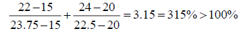
In Table 6, the right-hand side value of the first constraint is changed from 15,000 to 13,000; and the right-hand side value of the second constraint is changed from 20,000 to 17,000. The perturbations are in the same direction. If the ordinary 100% rule is applied the results of the 100% rule are:
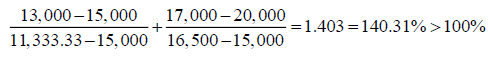
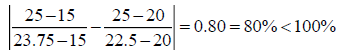
Hence the 100% rule is not satisfied and one may decide to resolve the problem. However, if we apply the modified 100% rule, by taking the absolute value of the subtraction, one gets:
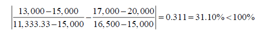
And the modified rule is satisfied. We find the following:
1. The optimal solution changes.
2. The total of the objective function value changes.
3. The ranges of optimality are the same.
4. The dual prices remain the same. Knowing the duals, the new level of the objective function can be calculated.
5. The slacks are changed.
6. The binding constraints remain binding.
7. The non-binding constraints remain non-binding.
8. The ranges of feasibility change.
Hence the modified rule has provided the correct results.
The right-hand side value of the third constraint is now changed from 20,000 to 25,000; and the right-hand side of the seventh constraint is now changed from 1,000 to 2,000. The perturbations are in the same direction. If the ordinary 100% rule is applied the results of the 100% rule are:
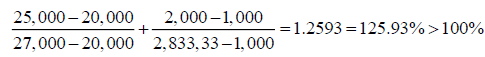
Hence the 100% rule is not satisfied and one may decide to resolve the problem. However, if we apply the modified 100% rule one gets:
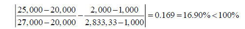
And the modified rule is satisfied, and the results support this assertion, and are not reported in a table. Hence, when perturbations are in the same direction the modified 100% rule must be applied. Otherwise a given optimal solution will be rejected.
This section applies one independent perturbation to the 4-variable minimization linear program. The right-hand side value of the first constraint is changed from 36 to 90; and the righthand side value of the third constraint is changed from 200 to 220.The perturbations from Table 7 are in the same direction. If the ordinary 100% rule is applied the results of the 100% rule are:
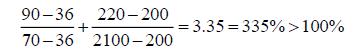
Hence the 100% rule is not satisfied and one may decide to resolve the problem. However, if we apply the modified 100% rule one gets:
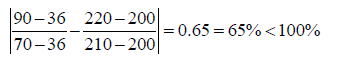
And the modified rule is satisfied. We find the following:
1. The optimal solution changes.
2. The total of the objective function value changes.
3. The ranges of optimality differ.
4. The dual prices remain the same. Knowing the changes in the coefficients, the new level of the objective function can be calculated.
5. The slacks are changed.
6. The binding constraints remain binding.
7. The non-binding constraints remain non-binding.
8. The ranges of feasibility change.
Hence the modified rule has provided the correct results.
Simultaneous perturbations in the coefficients of the objective function, and the modified 100% rule
This part will introduce two different optimization models in order to provide for a diversity of applications. One is a 3-variable maximization and the other is a 3-variable minimization. The maximization with three decision variables is as follows:
Maximize: 10X1+16X2+16X3
Subject to:
0.7X1+X2+0.8X3 ≤ 630
0.5X1+(5/6) X2+X3 ≤ 600
X1+(2/3) X2+X3 ≤ 708
0.1X1+0.25X2+0.25X3 ≤ 135
The 3-variable minimization is as follows:
Minimize: 15X1+15X2+20X3
Subject to:
X1+X3 ≤ 30
0.5X1+X2+6X3 ≥ 15
3X1+4X2+X3 ≥ 20
0.2X1+0.4X2+0.6X3 ≥ 5
Two such perturbations are implemented for each one of the 3-variable maximization, and for the 3-variable minimization. The results for the maximization are tabulated in Table 8 and the results for the minimization are tabulated in Table 9.
Table 8 THE 3-VARIABLE MAXIMIZATION LINEAR PROGRAM: THE FIRST PERTURBATIONS IN THE COEFFICIENTS OF THE OBJECTIVE FUNCTION |
||||||
| OPTIMAL SOLUTION | ||||||
| Objective Function Value=8579.6763020 | ||||||
| Variable | Value | Reduced Costs | ||||
| X1 | 403.7839042 | 0.0000000 | ||||
| X2 | 222.8105820 | 0.000 | ||||
| X3 | 155.6758563 | 0.000 | ||||
| Constraint | Slack/Surplus | Dual Prices | ||||
| 1 | 0.0000000 | 7.0270339 | ||||
| 2 | 56.7567140 | 0.000 | ||||
| 3 | 0.0000000 | 4.2162119 | ||||
| 4 | 0.0000000 | 8.6486441 | ||||
| OBJECTIVE COEFFICIENT RANGES | ||||||
| Variable | Lower Limit | Current Value | Upper Limit | |||
| X1 | 4.8000000 | 10.0000000 | 11.1428564 | |||
| X2 | 9.1111053 | 12.0000000 | 14.7368421 | |||
| X3 | 11.0000004 | 12.0000000 | 14.3636402 | |||
| RIGHT HAND SIDE RANGES | ||||||
| Constraint | Lower Limit | Current Value | Upper Limit | |||
| 1 | 538.4000000 | 630.0000000 | 682.3637319 | |||
| 2 | 543.2432860 | 600.0000000 | No Upper Limit | |||
| 3 | 579.9997200 | 708.0000000 | 852.6315789 | |||
| 4 | 116.9999764 | 135.0000000 | 151.1538354 | |||
| Table 9 THE 3-VARIABLE MINIMIZATION OF THE LINEAR PROGRAM: THE FIRST PERTURBATIONS IN THE COEFFICIENTS OF THE OBJECTIVE FUNCTION |
||||||
| OPTIMAL SOLUTION | ||||||
| Objective Function Value=237.500 | ||||||
| Variable | Value | Reduced Costs | ||||
| X1 | 0.000 | 0.000 | ||||
| X2 | 3.500 | 0.000 | ||||
| X3 | 6.000 | 0.000 | ||||
| Constraint | Slack/Surplus | Dual Prices | ||||
| 1 | 24.000 | 0.000 | ||||
| 2 | 24.500 | 0.000 | ||||
| 3 | 0.000 | -2.500 | ||||
| 4 | 0.000 | -37.500 | ||||
| OBJECTIVE COEFFICIENT RANGES | ||||||
| Variable | Lower Limit | Current Value | Upper Limit | |||
| X1 | 15.000 | 15.000 | No Upper Limit | |||
| X2 | 16.667 | 25.000 | 25.000 | |||
| X3 | 25.000 | 25.000 | 37.500 | |||
| RIGHT HAND SIDE RANGES | ||||||
| Constraint | Lower Limit | Current Value | Upper Limit | |||
| 1 | 6.000 | 30.000 | No Upper Limit | |||
| 2 | No Lower Limit | 15.000 | 39.500 | |||
| 3 | 8.333 | 20.000 | 47.222 | |||
| 4 | 2.870 | 5.000 | 12.000 | |||
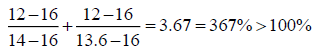
The second and third coefficients in the objective function of the 3-variable maximization program are changed respectively from 16 to 12, and from 16 to 12. The perturbations are in the same direction. If the ordinary 100% rule is wrongly applied the results of the 100% rule are:
Hence the 100% rule is not satisfied and one may decide to resolve the problem. However, if we apply the correct modified 100% rule one gets:
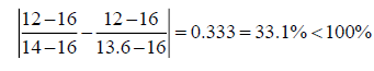
And the correct modified rule is satisfied. We find the following:
1. The optimal solution does not change.
2. The total of the objective function value changes and can be calculated.
3. The ranges of optimality change.
4. The dual prices change.
5. The slacks are the same.
6. The binding constraints remain binding.
7. The non-binding constraints remain non-binding.
8. The ranges of feasibility do not change.
Hence the modified rule has provided the correct results.
The first and third coefficients of the objective function of the 3-variable maximization program are changed respectively from 10 to 16, and from 16 to 19. The perturbations are in the same direction. If the ordinary 100% rule is wrongly applied the results of the 100% rule are:
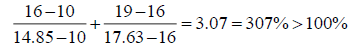
Hence the 100% rule is not satisfied and one may decide to resolve the problem. However, if we apply the correct modified 100% rule one gets:
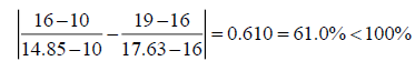
And the correct modified rule is satisfied. We find the same results as above, and will not be repeated. Hence the modified rule has provided the correct results.
The second and third coefficients of the objective function of the 3-variable minimization program are changed respectively from 15 to 25, and from 20 to 25. The perturbations are in the same direction. If the ordinary 100% rule is wrongly applied the results of the 100% rule are:
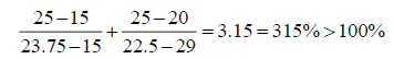
Hence the 100% rule is not satisfied and one may decide to resolve the problem. However, if we apply the correct modified 100% rule one gets:
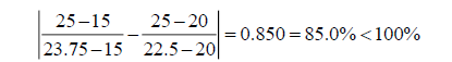
And the correct modified rule is satisfied. We find the following:
1. The optimal solution does not change.
2. The total of the objective function value changes and can be calculated.
3. The ranges of optimality change.
4. The dual prices change.
5. The slack/surplus is the same.
6. The binding constraints remain binding.
7. The non-binding constraints remain non-binding.
8. The ranges of feasibility do not change.
Hence the modified rule has provided the correct results.
The second and third coefficients of the objective function of the 3-variable minimization program are now changed respectively from 15 to 22, and from 20 to 24. The perturbations are in the same direction. If the ordinary 100% rule is wrongly applied the results of the 100% rule are:
Hence the 100% rule is not satisfied and one may decide to resolve the problem. However, if we apply the correct modified 100% rule one gets:
And the correct modified rule is satisfied. We find the same results as above, and will not be repeated. Hence the modified rule has provided the correct results.
Conclusion
To summarize, this paper envisaged one essential part of linear programming models, and which is sensitivity analysis, also called post-optimality analysis because it starts from and builds upon the original optimal solution. Many systematic perturbations were applied to the original set-ups. One of them was to multiply the objective function threefold. The choice of 3 is arbitrary and other values work as well. Another was to multiply the right-hand side coefficients of the constraints threefold, which is, again arbitrary, but does not materially affect the analysis. Then, simultaneous perturbations were subjected to the models. A crucial shortcoming of the 100% rule, as reported in textbooks, is discovered. In its place the author has suggested to modify the rule. This modification works well in most circumstances. One important part of the analysis is when the modified 100% rule is satisfied. In this case either the solution remains optimal, or the dual prices do not change. The former applies to simultaneous perturbations in the objective value coefficients, and the latter to simultaneous perturbations in the right-hand side variables of the constraints. The purpose of the paper is to encourage critical thinking in linear programming and to offer practical solutions that are easy and straightforward. One avenue for future research is to demonstrate mathematically why the modified 100% rule works so well.
References
- Anderson, D.R., Sweeney, D.J., Williams, T.A., Camm, J.D., Cochran, J.J., Fry, M.J., & Ohlmann, J.W. (2016). An introduction to management science: Quantitative approaches to decision making, (Fourteenth Edition), Thomson South‐Western CollegePublishing, Cengage Learning.
- Bradley, S.P., Hax, A.C., & Magnanti, T.L. (1977). Applied mathematical programming. AddisonWesley.
- Dorfman, R., Samuelson, P.A., & Solow, R.M. (1958). Linear programming and economic analysis. New York: McGraw‐Hill
- Filippi, C. (2011). Sensitivity analysis in linear programming. In John J. Cochran (ed.), Wiley Encyclopedia of Operations Research and Management Science. Wiley,
- Ward, J.E., & Wendell, R.E. (1990). Approaches to sensitivity analysis in linear programming. Annals of Operations Research, 27(1), 3‐38.