Keywords

Retirement Model, Constant Savings Rate, Real Income Growth, Retirement, Retirement Planning, Retirement Goals, Retirement Savings.

Literature Review

Lown (2008) provides an extensive review of the baby boom generation savings adequacy literature that reveals that one-half of the baby boomers will be able to continue their preretirement standard of living, while the other half may face challenges that range from moderate to severe, even to the point of poverty. For some, inadequate preparation for retirement could be linked to financial illiteracy.

In the 2016 Employee Benefit Research Institute’s Retirement Confidence Survey, employee confidence in being able to provide a comfortable retirement improved slightly from the 2015 survey results: (1) Very confident 21% (22% in 2015); (2) Somewhat confident 42% (36% in 2015); (3) Not too confident 16% (17% in 2015); and, (4) Not at all confident 19% (24% in 2015). The improvement in retirement confidence in 2015 (after confidence lows in 2009-2013) was attributed to participation in a retirement plans (Helman et al., 2016). Regardless of the improvement, 36% of the 2016 survey respondents are either not too confident or not at all confident of being prepared for a comfortable retirement.

Several authors have discussed financial literacy and retirement preparedness, and proposed ways in which employers can help employees, young and old, prepare for retirement and reduce the risk of outliving retirement assets (Christman, 2010; Lusardi & Mitchell 2007). Some organizations have provided online tools to help individuals improve their financial literacy; for example, American Institute of Certified Public Accountants’ 360 degrees of Financial Literacy, and, Standard and Poors’ Financial Literacy Now. Lown (2008) recommends less debate over the percent at risk or the measurement of retirement adequacy and more research on solutions for helping individuals make better decisions given their individual circumstances.

Gustafson et al. (2005) developed a retirement model that, given certain assumptions, would provide the percent of income that an investor would need to save (the savings rate) during his pre-retirement years in order to provide for a comfortable retirement. According to Gustafson et al. (2005), a stream of research related to estimating the financial resources is needed for retirement which often involves a ratio of retirement needs frequently referred to as the replacement rate. While this ratio will vary depending on each individual’s circumstances, a replacement rate of 70% of his or her current salary is a common guideline. The 70% replacement rate is applicable to a wide range of income groups, with a higher rate required of lower income groups, and a lower rate for higher income groups (McManus et al., 2008). For purposes of determining a replacement rate, each individual needs to consider other sources of income, lower tax rates, and typically less expenses, such as food, clothing, and commuting. One stated limitation of their model was that the income was adjusted for inflation each year, but real increases in income during the pre-retirement years were not included. This paper extends their model by including an increase in the real income variable during the pre-retirement period and eliminating the need to forecast inflation.

Over the years, research has focused on past savings rates in the United States, as well as, proposed future safe savings rates. Using wealth survey data from 1984 through 1994, Gist et al. (1999) studied the retirement saving adequacy of the Baby Boomer generation classifying by older or younger boomers, single or married, and with or without pension. Assuming a 3.9% real rate of return, they found that the needed saving rates for younger boomers (born 1955-1964), married, with a pension ranged from 2.6% to 8.6%, while without a pension, they ranged from 5.8% to 15.5%.

Pfau (2011) claimed that traditional retirement planning often focuses on a targeted accumulated amount at retirement using a retirement multiple. For instance, one might assume a 4% withdrawal amount and a 50% replacement of final salary. A retirement multiple of 12.5 is calculated by dividing the 50% replacement rate with the 4% withdrawal rate. The 12.5 would then be multiplied by the person’s final salary. By planning for retirement in this fashion, the working (accumulation) and the retirement (decumulation) phases are not considered together. Rather than focusing on the withdrawal rate, Pfau found that focusing on a “safe savings rate” for eighty overlapping sixty year life cycles (thirty years working and thirty years retired) using annual financial asset returns from 1871 - 2009, provided enough accumulated wealth to cover the required retirement expenditures, even though 59% of the rolling thirty year work periods resulted in accumulated amounts less than 12.5 times the final salary. A limitation of this “safe saving rate” determination is that it relies on historical data. Goebel & Zivney (2014) extended the research done by Pfau (2011) and found on average a safe savings rate to be 14% when considering 30 years working, 30 Year retirement, and social security providing 50% of retirement needs.

Also to be considered is the issue of the cost of long term care, which is related to longevity. This cost is a large expenditure risk for the elderly (Brown et al. 2012), with almost 20% of persons age 65 and older having care at a long-term facility for two or more years (Kemper 2005). Nursing home costs average over $75,000 per year (Inglehart, 2010), with costs even more if the care is in a small group home or at the private home of the individual receiving the care. If an individual does not have long term care insurance, they need to consider this cost as part of the amount they need to accrue for retirement.

Samavati et al. (2013) studied the personal savings rate as a percentage of disposable income in the United States, and they noted that it had been declining for two decades from 10.9% in 1982 to 1.4% in 2005. However, the trend has reversed since the Great Recession in 2007, with savings rates gradually increasing from 2.1% in 2007 to 5.7% in 2010. The authors attribute this to increase to a reduction in net wealth. While, the personal savings rate has gradually increased, 5.7% in 2010 falls short of some of the recommended retirement adequacy savings rates needed in the previously mentioned research.

The Model

The objective of this paper is to propose a retirement model to further the realism of existing models, i.e., the Gustafson et al. model, by including as a variable the real growth of income. In developing the model, ease of implementation and use was a priority. As a result, the output of the model is a value representing the percentage of income that must be invested during the savings period. This value is to remain constant even if income increases due to real increases in income.

The need to incorporate the real growth in income responds to the fact that when an individual begins to work and save for retirement, the type of job and its corresponding compensation is not usually the same type of job that the individual holds just before retirement. Income increases with inflation, but also with increases in real salary because of promotions due to more and/or higher responsibilities. As a result, the growth in income during the working years is higher than the inflation rate.

In the Gustafson et al. model, the growth in income is the same as the inflation rate, implying that the real growth in income is zero. Use of their model may result in overestimation of the savings rate, since it ignores increases in real income. Our model differentiates between inflation and growth in real income. Another difference is that the Gustafson model considers only one rate of return, while our model considers three different rates of return, one for the savings period, another for the retirement period, and another for the previously accumulated assets directed toward generating retirement income in the future.

The consideration of inflation and real growth in income as separate variables makes the model more realistic. However, inflation is not an explicit variable in our model. As such, as will be illustrated later, it does not need to be estimated. It is implicitly part of the model during the savings and retirement phases, since inflation impacts the income on which the savings rate is applied and also the amounts needed for withdrawal in the future. During the savings phase, the savings rate is applied on an income that is increasing due to inflation and other factors that make the real growth rate higher than zero. During the retirement phase, the amount to be withdrawn may be adjusted by past actual inflation rates in order to keep its acquisition power constant.

The model allows for the inclusion of assets already accumulated at the time of planning. This characteristic permits the savings rate to be reviewed and adjusted if there are differences between the sizes of the planned and actual fund. This difference may be caused by variation in return rates and income and also by changes in retirement goals. The impact of increased life expectancy during the savings period (and the related possibility of long term care costs) may be another reason to adjust the savings rate.

The model is based on known time value of money equations. It was developed in three steps, in a sequential manner, to aid in its understanding. First, it is assumed that there is no growth in income, and that inflation is zero. These two assumptions make it easy to understand the basics of the model. Growth in real income and no inflation are considered next. Finally, growth in real income and inflation are incorporated in the model. The appendix presents the development of the model.

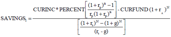
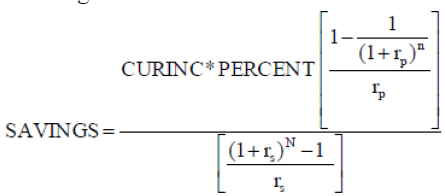
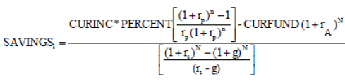
The following equation summarizes the first part of the model, which is to calculate the amount of savings: expenses.

(1)

Where:

SAVINGS₁ = annual amount to save at the end of period one

CURINC = current annual income

PERCENT = percent of current income desired as pension (replacement rate)

CURFUND = accumulated assets at time of planning

g = expected annual real growth rate in annual income

rp = expected annual real return during retirement period

rs = expected annual real return during savings period

rA = expected annual real return for accumulated assets

n = number of years in retirement

N = number of years during savings period

Subject to rs > g.

In the following periods the savings amount (SAVINGS₁) will be adjusted by the growth rate of income (g). If g = 0, the savings amount remains constant.

The numerator of the equation corresponds to the accumulated amount to be saved at the end of the savings period. The second part of the numerator, CURFUND (1+ rA)^N, is the value at the time of retirement of the of the accumulated assets at the time of planning.

After a number of years, the accumulated savings (the fund) may not be what it is forecast to be. One of the reasons could be that the real return was not what it was forecast to be. This would be one reason to revise the savings rate on a periodical basis to make necessary adjustments to the amount being saved. The second part of the numerator in equation (1) allows for this adjustment.

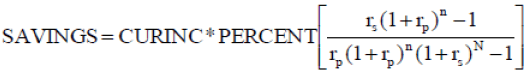
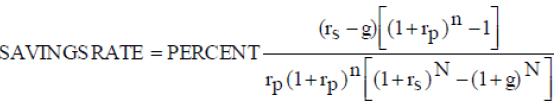
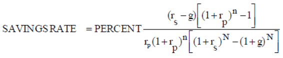
The second part of the model is obtaining a savings rate (SAVINGSRATE). To obtain a savings rate the savings amount (SAVINGS1) obtained with equation (1) is divided by current income (CURINC).

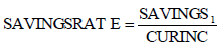(2)

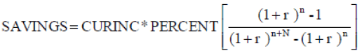
If just one equation is needed, the savings rate may be obtained by dividing both sides by the current income (CURINC) resulting in a constant savings rate. The following equation summarizes the entire model:

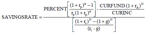(3)

The savings rate will be constant since, by construction, income increases at the same rate that the savings amount increases by. As can be seen (or not be seen) inflation is not a variable. As can be observed in the Appendix, the inflation rate is introduced, but it is eliminated in the derivation of the model. Since the savings rate is applied on annual income, the annual savings amount will be adjusted if nominal income increases.

The fact that no inflation rate needs to be used as input simplifies and improves the usability of the model. There is no need to forecast inflation; just to enter an estimated real rate of return for the savings and retirement periods. We believe that the volatility of real rates of return is lower than the volatility of nominal rates of return. Consequently, forecasting real rates of return is subject to less errors than forecasting nominal rates of return.

The other important variable is a real growth rate for income. This rate can be estimated considering beginning and ending current incomes for jobs or professions.

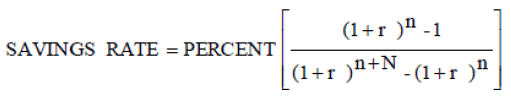
If the return rates for the savings and retirement periods are the same and there is no accumulated assets, equation (3) becomes:

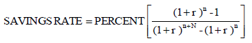(4)

No dollar amounts are needed, just the planned years of working and retirement and a common rate of return for both periods.

Illustrations Using the Model

The following examples illustrate the use of the model:

Illustration 1 - Constant Income

For this illustration, in addition to social security and other income, an individual wants to receive 100% of his current income of $36,000 for 20 years after retiring with funds generating 4% annually. He plans to work for 35 years. Applying equation (1), the individual needs to save $6,642.73 each year. After applying formula (2), this represents 18.45% of his current income. A longer savings (and working) period and a shorter retirement period will lower this amount. Table 1 shows the percentage of income depending on whether the individual works for 30, 35 or 40 years, and whether he lives for 15, 20 or 25 years after retiring. The savings rates shown in the table above could have been obtained using equation (4).

Table 1 Saving Rates With no Real Growth in Income and no Inflation
Retirement Years	Work Years
	30	35	40
15	20%	15%	12%
20	24%	18%	14%
25	28%	21%	16%

The minimum percentage of income is 12% (40 work years and 15 retirement years), and the maximum is 28% (30 work years and 25 retirement years). In any case, at the end of the retirement period, the fund will be depleted.

Illustration 2 - Growth in Real Income

Using equation (1) and information from the previous example, and assuming a real income growth of 3% per year, the amount to be saved in the first year is $4,321.35. Applying equation (2) results in a savings rate of 12.00% of current income. This percentage will remain constant throughout the working period. As the income increases, the amount saved will increase. For example, in the second year, the amount saved will increase by 3%, which is the increase in real income. Inflation is assumed to be zero.

An interesting result is that at the end of the working period (year 35) the worker’s income in real terms will be $101,299 (due to the 3% growth), while his pension will be just $36,000 which is 100% of his current income when he starts to save, but just 35% of his final income. The percentage applied on current income should contemplate real incomes at the end of the savings period. Higher desired pensions will require higher savings rates.

Table 2 shows the savings rates when real income is expected to grow at 3% per year. The number of years to work are 30, 35 or 40 and retirement periods are 15, 20, or 25 years.

Table 2 Saving Rates with Real Growth in Income
Retirement Years	Work Years
	30	35	40
15	14%	10%	7%
20	17%	12%	9%
25	19%	14%	10%

Comparing Table 1 to Table 2 the percentages of income to be saved for retirement are lower, as expected, in all instances.

The 3% used as the real growth rate in income in the current illustration was arbitrarily chosen. A common user will likely not be able to calculate a growth rate between beginning and ending current income given a number of years, but he would have an idea of the number of times his expected ending income is relative to his current income. Table 3 shows estimated growth rates based on multiples of ending income to current income depending on the length of the savings (working) period.

Table 3 Income Growth Rates at Diff. Multiples and Savings Periods
	Savings Period (Years)
Multiple	20	25	30	35	40
2	3.5%	2.8%	2.3%	2.0%	1.7%
3	5.6%	4.5%	3.7%	3.2%	2.8%
4	7.2%	5.7%	4.7%	4.0%	3.5%
5	8.4%	6.6%	5.5%	4.7%	4.1%

For example, if a college graduate expects his income before retirement in current dollars to be three times his current income after 35 years of work, he will use a growth rate of 3.2% or just 3%.

Illustration 3 - Including Differential Rates of Return

The same parameters are used, but the rate of return for the fund during the retirement period is not 4%, but 2%. This lower rate reflects the fact that, during the retirement period, the rate of return could be more conservative. The resulting savings rate increases to 14.44%. Since the rate of return for the retirement period is a factor in the denominator, the equation doesn’t allow for an input of 0%. This limitation is overcome by entering a value close to 0% (i.e.: 0.0001%).

Illustration 4 - Including Accumulated Assets

The same parameters used in the previous illustrations are used here as well. The difference now is that the user has inherited $50,000 and would like to consider this asset in his retirement planning. Using 4% as the rate of return, for both the savings and retirement periods, the $50,000 becomes $197,304.45 after 35 years (just before retirement). No growth in real income is assumed, and consequently there is no growth in the amount being saved. The result is that he needs to save only $489,251.45. The required savings per year is $2,578.52, which is 7.16% of his current income.

Retirement Plan Adjustments

Equation (1) can also be used to adjust the savings rate when time has passed, and a review and an update of the retirement plan is called for, because of possible changes in desired pension, changes in household conditions or just to check if the current savings rate will lead to the planned retirement fund.

Changes in economic conditions may affect the real return. It may not be what it was forecast to be. That would be one reason to revise the savings rate on a periodical basis to make necessary adjustments in the amount being saved.

Illustration 5 - Retirement Plan Adjustments

Assume that the individual savings for retirement planned as shown in Illustration 1. His plan called for 35 years of work, a 18.45% savings rate (with respect to his current income) at a 4% return and a $36,000 retirement pension for 20 years. To avoid complexity, no real increase in income and no inflation are assumed.

It has been 10 years since the individual used the model. His annual income is $36,000. It has been constant. He is saving 18.45% of his annual income. It is now the end of Year 10, and he has just made the corresponding savings deposit and realizes that his fund’s balance is $60,000 instead of being $79,753.31 as forecast when he began to save. Evidently, the return rate of his fund has not been 4% in real terms, or he has not saved 18.45% of his annual income.

The model can be used to recalculate the percentage he needs to save now, and into the future, to reach his retirement goal. He has 25 more years of savings (25 more years of work) and uses a 4% real rate of return in his calculations for the return during both the working and retirement years. He still wants a $36,000 pension and plans to live 20 years in retirement. After these parameters are entered in the model (equation 1), the result is that he should save $7,907.18 annually, which represents 21.96% of his income starting the following year. (If the amount that he planned before to accumulate at this point ($79,753.31) is entered as assets already accumulated, the resulting percentage savings will be the original savings rate (18.45%).

Since this seems a little too high, he wants to see how much it will be if, instead of working 25 more years, he works 30 more years. After entering the required information, the model predicts that he should save $5,263.60 which represents 14.59% of his annual income.

The Role of Inflation

As mentioned before, inflation or, actually, expected inflation, is not an explicit variable in the model. However, inflation will impact the annual income and the corresponding savings amount, and consequently, the size of the fund after the working years. This in turn will impact the periodic amounts to be withdrawn in the future to keep up with the cost of living.

To illustrate that inflation doesn’t need to be considered explicitly in the model, equation (1) was used under four different scenarios with equal incomes at the beginning of the savings period, equal pensions at retirement and, also, the same number of working and retirement years. The objective was to show that, with and without inflation, the savings rate is the same.

In all four scenarios, the beginning income is the same, the replacement rate is 100%, the savings period is 35 years, the retirement period is 20 years, and the rate of return for the fund is 4%, for both the savings and the retirement periods. The annual real growth in income was assumed to be 3%, and the annual inflation rate is also 3%.

The difference in the four scenarios are the real growth in income and the inflation rate. In Scenario One there is no real income growth and no inflation. In Scenario Two, there is no real income growth, but there is inflation. In Scenario Three, income grows in real terms, but there is no inflation. Finally, in Scenario Four, there is a combination of real income growth and inflation. Table 4 shows the parameters used in each of the four scenarios.

Table 4 Parameters Used In Scenarios 1-4
	Scenario One	Scenario Two	Scenario Three	Scenario Four
	No Growth/No Inflation	No Growth/ Inflation	Growth/ No Inflation	Growth/ Inflation
Current income ($)	35,000	35,000	35,000	35,000
Pension desired (as % of income)	100%	100%	100%	100%
Number of years to work and save	35	35	35	35
Number of years to live in retirement	20	20	20	20
Annual real rate of return (%)	4.00%	4.00%	4.00%	4.00%
Annual real growth rate of income (%)	0.00%	0.00%	3.00%	3.00%
Annual inflation rate (%)	0.00%	3.00%	0.00%	3.00%

The results are presented in Table 5. Row wise, the table shows the savings rate for each scenario, the beginning and ending incomes and savings, the fund size at retirement, and the beginning and ending pensions. The annual pension in real terms is the same in all four scenarios.

Table 5 Scenarios 1-4 Results Using the Model
Item	Scenario One	Scenario Two	Scenario Three	Scenario Four
	No Income Growth	No Income Growth	Income Growth: 3.0%	Income Growth: 3.0%
	No inflation	Inflation: 3.0%	No inflation	Inflation: 3.0%
Savings Rate (% of Cur.Inc.)	18.45%	18.45%	12.00%	12.00%
Beginning Annual Inc. ($)	35,000	35,000	35,000	35,000
Ending Annual Inc. ($)	35,000	95,617	95,617	261,216
Beginning Annual Savings ($)*	6,458	6,458	4,201	4,201
Ending Annual Savings ($)	6,458	17,643	11,477	31,354
Fund Size at Retirement ($)	475,661	1,299,462	475,661	1,299,462
Beginning Pension ($)	35,000	98,485	35,000	98,485
Ending Pension ($)	35,000	172,694	35,000	172,694

The savings rate calculated with the model was applied on the annual incomes in each of the scenarios. The inflation rate was used to calculate the annual incomes and savings during the savings period, and also the annual pensions during the retirement period. In addition, it was used to calculate the size of the fund during the savings and retirement periods.

The figures shown in the table confirm that inflation is not a variable that needs to be estimated and input in the model. The savings rate is 18.45% when there is no growth in real income, with and without inflation, and 12% when the growth is 3% per year, with and without inflation.

The following points are worth noting:

1. Given a growth in real income, the savings rate is the same regardless of the inflation rate.

2. The savings rate is lower in the presence of real income growth.

3. Given a growth in real income, the amounts to be saved each year are the same, regardless of the inflation rate.

4. The amount to be saved each year is constant only in the first scenario (no income growth, no inflation).

5. Ending income increases as the scenarios include real income growth or inflation, or the combination of both.

6. The fund size at retirement is higher in the scenarios with inflation. Real income growth doesn’t play any role in the final size of the fund.

7. The beginning and ending pensions are impacted by inflation, not by increase in real income.

8. The resulting beginning and ending pensions in all four scenarios are the same in real terms.

As shown in equation (1) and illustrated in the previous section, inflation is not a variable in the model. It does not need to be entered and, consequently, it does not need to be estimated. However, it is not easy to grasp the idea that inflation is not a factor and that no adjustments need to be made to the resulting savings rate during the savings period. Inflation is only used in the retirement period in order to adjust the pension to keep the acquisition power constant.

We further illustrate the fact that inflation is not a variable in the model, displaying how the fund is built during the savings period, and how it is depleted during the retirement period, when pensions are withdrawn, reaching a value of zero at the end of the planned retirement period. The values used are the same used in preparing Table 5.

We present the results in two sections comparing two pairs of scenarios (Scenarios One and Two and Scenarios Three and Four). In each pair, the growth in real income is the same. Within the pair, the difference is the inflation rate.

No Growth in Real Income

Table 6 shows figures for Scenarios One and Two. In both cases there is no real growth in income. In Scenario One, there is no inflation, whereas in Scenario Three, an inflation rate of 3% impacts the annual income, the rate of return, the savings and pension amounts, and the fund’s size. However, in both scenarios, the savings rate is the same (18.45%). In both cases the annual savings amounts are able to build a fund by the end of the savings period that can later sustain the desired pension and be reduced to zero at the end of the planned retirement period.

Table 6 No Growth in Real Income
SCENARIO ONE- REAL INCOME GROWTH: 0% - INFLATION: 0%						SCENARIO TWO - REAL INCOME GROWTH: 0% - INFLATION: 3%
SAVINGS PERIOD						SAVINGSPERIOD
PER	INCOME	BEG BAL	RETURN	SAVINGS	END BAL	PER	INCOME	BEG BAL	RETURN	SAVINGS	END BAL
1	35,000	-	-	6,458	6,458	1	35,000	-	-	6,458	6,458
2	35,000	6,458	258	6,458	13,175	2	36,050	6,458	460	6,652	13,570
3	35,000	13,175	527	6,458	20,160	3	37,132	13,570	966	6,852	21,388
:		:	:	:	:	:		:	:	:	:
33	-	404,939	6,458	16,198	427,595	33	-	1,012,380	16,630	72,081	1,101,092
34	-	427,595	6,458	17,104	451,157	34	-	1,101,092	17,129	78,398	1,196,619
35	-	451,157	6,458	18,046	475,661	35	-	1,196,619	17,643	85,199	1,299,462
RETIREMENT PERIOD						RETIREMENT PERIOD
PER		BEG BAL	RETURN	PENSION	EB	PER		BEG BAL	RETURN	PENSION	END BAL
1		475,661	19,026	(35,000)	459,688	1		1,299,462	92,522	(98,485)	1,293,498
2		459,688	18,388	(35,000)	443,075	2		1,293,498	92,097	(101,440)	1,284,156
3		443,075	17,723	(35,000)	425,798	3		1,284,156	91,432	(104,483)	1,271,105
:		:	:	:	:	:		:	:	:	:
18		97,128	3,885	(35,000)	66,013	18		438,575	31,227	(162,781)	307,020
19		66,013	2,641	(35,000)	33,654	19		307,020	21,860	(167,664)	161,216
20		33,654	1,346	(35,000)	0	20		161,216	11,479	(172,694)	0

The top section of the table shows the amounts being saved (SAVINGS) and accumulated in the retirement fund (END BAL) during the savings period. The amounts being saved are the result of multiplying the savings rate (18.45%) times the current income. Due to inflation, this amount is constant in Scenario One and increasing in Scenario Two.

The bottom section shows the amount being paid as pension (PENSION) and the balance of the retirement fund (END BAL) during the retirement period. Due to inflation, this amount is constant in Scenario One and increasing in Scenario Two.

Growth in Real Income

Table 7 shows figures for Scenarios Three and Four. In both cases, real income increases by 3% in real terms. In Scenario Three, there is no inflation, whereas in Scenario Four, an inflation rate of 3% is considered. The savings rate in both cases is the same (12%). The structure of this table is the same as Table 6.

Table 7 Growth in Real Income
SCENARIO THREE - REAL INCOME GROWTH: 3% - INFLATION: 0%						SCENARIO FOUR - REAL INCOME GROWTH: 3% - INFLATION: 3%
SAVINGS PERIOD						SAVINGS PERIOD
PER	INCOME	BEG BAL	RETURN	SAVINGS	END BAL	PER	INCOME	BEG BAL	RETURN	SAVINGS	END BAL
1	35,000	-	-	4,201	4,201	1	35,000	-	-	4,201	4,201
2	36,050	4,201	168	4,327	8,696	2	37,132	4,201	299	4,457	8,957
3	37,132	8,696	348	4,457	13,501	3	39,393	8,957	638	4,728	14,323
:		:	:	:	:	:		:	:	:	:
33	-	391,954	10,818	15,678	418,450	33	-	979,916	27,858	69,770	1,077,544
34	-	418,450	11,143	16,738	446,331	34	-	1,077,544	29,554	76,721	1,183,820
35	-	446,331	11,477	17,853	475,661	35	-	1,183,820	31,354	84,288	1,299,462
RETIREMENT PERIOD						RETIREMENT PERIOD
PER		BEG BAL	RETURN	PENSION	END BAL	PER		BEG BAL	RETURN	PENSION	END BAL
1		475,661	19,026	(35,000)	459,688	1		1,299,462	92,522	(98,485)	1,293,498
2		459,688	18,388	(35,000)	443,075	2		1,293,498	92,097	(101,440)	1,284,156
3		443,075	17,723	(35,000)	425,798	3		1,284,156	91,432	(104,483)	,271,105
:		:	:	:	:	:		:	:	:	:
18		97,128	3,885	(35,000)	66,013	18		438,575	31,227	(162,781)	307,020
19		66,013	2,641	(35,000)	33,654	19		307,020	21,860	(167,664)	161,216
20		33,654	1,346	(35,000)	0	20		161,216	11,479	(172,694)	0

As in Scenarios One and Two, the savings amounts are different due to inflation, but in real terms they are the same. Changing the inflation rate in Scenario Four will yield the same result. That is, the annual savings will be enough to build a fund that will sustain the desired annual pensions during the retirement period.

Summary Notes on the Model

Inflation doesn’t play any role in the model. It may impact nominal rates of return and nominal income and consequently savings, fund size, and pension, but it does not need to be estimated. Only real rates are needed.

Table 8 lists the sets of values used in the previous four examples, including their annual nominal equivalents. The last row shows the resulting savings rates, obtained using equation (1). As can be seen, the savings rates are the same regardless of the inflation rates. As expected, the savings rates are lower in the presence of real growth in income.

Table 8 Summary
Summary	Scenario One	Scenario Two	Scenario Three	Scenario Four
	No Growth/No Inflation	No Growth/Inflation	Growth/ No Inflation	Growth/Inflation
Real rate of return	4.00%	4.00%	4.00%	4.00%
Real growth in income	0.00%	0.00%	3.00%	3.00%
Annual Inflation Rate	0.00%	3.00%	0.00%	3.00%
Nominal rate of return	4.00%	7.12%	4.00%	7.12%
Nominal growth in income	0.00%	3.00%	3.00%	6.09%
Resulting savings rate	18.45%	18.45%	12.00%	12.00%

Using the Model in Excel

Table 9 shows a screen capture of the model in Excel. Cells B1 to B10 contain the parameters. Cell B12 contains the formula to estimate the savings in the first year. If there is no growth in real income and no inflation, this savings amount will be constant until retirement. Cell B13 contains the formula to estimate the savings rate. Cell B14 contains the formula to estimate the fund’s size.

Table 9 Model Parameters - Excel Screenshot
	A	B
1	PARAMETERS
2	Current Income (CURINC)	35,000
3	% of current income desired as pension	100%
4	Number of years during savings period (N)	35
5	Number of years in retirement (n)	20
6	Annual real rate of return during savings period (rs)	4.00%
7	Annual real rate of return during retirement period (rp)	4.00%
8	Real growth rate of annual income (g)	3.00%
9	Current assets (CURFUND)	0
10	Annual real rate of return of current assets (rA)	4.00%
11	RESULTS
12	Annual amount to save at the end of period one (SAVINGS1)	4,201
13	% of current income	12.00%
14	Size of fund at end of savings period	475,661

Amount to Save Each Year

The formula in cell B12 is as follows:=(B2*B3*((1+B7)^B5-1)/(B7*(1+B7)^B5)- B9*(1+B10)^B4)/(((1+B6)^B4-(1+B8)^B4)/(B6-B8)). This formula corresponds to Appendix equation (1). It is important that the parentheses be entered as indicated.

Savings Rate

The formula in cell B13 is as follows: =B12/B2. It corresponds to the savings rate. The savings rate could have been calculated using equation (3).

Fund Size

The formula in cell B14 is as follows:=(B2*B3*((1+B7)^B5-1)/(B7*(1+B7)^B5)- B9*(1+B10)^B4). This formula corresponds to the numerator in equation (1).

Advantages of the Model

Calculation of a Savings Rate, Not a Savings Amount

Using a savings rate applied on an income is better than using a specified dollar amount, since the latter will not keep up with changes in income. The required savings to build a retirement fund is stated as a percentage figure. As such, it is independent of the annual income level in dollar amounts and remains constant throughout the savings period, even when real income increases. The only other variables affecting the percentage are the number of work years, the number of years in retirement and the real return.

Inflation is Not a Component Variable

Thus, there is no need to forecast inflation. The assumption is that inflation will impact real income and real return by the same rate: i.e., if inflation is 5%, real return will be increased by 5% and current income will also be increased by 5%. Consequently, the savings rate (percentage of income) will not change. If inflation impacts the increase in income and rate of return at different rates, equations (1) and (2) can be used to adjust the savings rate and guarantee the required fund size. The savings amount will be automatically adjusted since the savings rate will be applied on an income that has been adjusted for real growth and inflation. However, at withdrawal, the pension will need to be manually adjusted by the inflation rate. For ease of adjustment, past actual inflation rates may be used.

Growth in Real Income is a Model Component

Real income increases are included in the model. Increases in income may be caused by inflation, but they may also be the result of increases in real income as a result of promotion, more experience, more knowledge, responsibility, etc. Expected real rate of return is used and there is no need to enter expected inflation or expected nominal rates of return.

If increases in real income do not occur as projected, equations (1) and (2) can periodically be used to adjust the savings rate. The adjustments will be smaller than if nominal rates were used, since inflation rates show more volatility than real rates. Increases in real income are not as difficult to forecast as inflation rates. In any case, the range of real values to choose from is narrower than those in the nominal range.

Current Assets may be Considered

The proposed model also considers the possibility of incorporating any accumulated savings or existing assets that are to be used for retirement purposes. These assets can be invested at their own real rate or return.

This characteristic makes the model versatile, because the user can check the status of their fund at any time, and adjust their savings rate depending on their accumulated retirement fund, expected future behavior of their real income, and real rates of return.

Differential Real Rates of Return may be Used

One can be used during the savings period and another for the retirement period. The latter allows the adoption of a conservative position. Also, a different real rate of return may be used for accumulated assets at the time of planning.

Risk can be Addressed

By using Excel capabilities, what if scenarios can be constructed assuming different rates of return.

Limitations of the Model

Real Rates of Return are Not Observable

Another limitation of the model is that the user has to enter the real rate of return on his savings or investments. This information is not observable. Only estimates of the real rate can be entered. The limitations given could be significant. Forecasting rates of return is subject to errors, but the variability of real rates of return is lower than the variability of nominal rates of return.

Real Rates of Growth in Income are Not Observable

If the individual is to take advantage of the model in the sense that expected increases in real income results in lower savings rates, he needs to enter an estimate of a real growth rate of income. Even if he knows ending annual incomes applicable to his conditions, he may not know how to estimate a real growth rate for his income. However, he may have an idea of the number of times his expected ending income might be with respect to his current income. He may then examine the table (Table 3) shown in this paper

Before the End of the Retirement Period the Fund may be Depleted

The model works well during an individual’s working period, because the user can calibrate his savings depending on the current size compared to the projected size of his retirement fund, the rates of return, the real rate of his increase in income and changes in the working and retirement periods. However, as with any other retirement model, once the individual stops working and saving, and starts living off his retirement fund, there is no guarantee that the fund will be enough to sustain his living expenses.

One factor that may affect his future pensions is the rate of return generated by his retirement fund. The rate of inflation can also impact his expenses in a way that exceeds the way it impacts the real rates of return. The response to this limitation is to use a very low rate of return, or even a negative one for the retirement period, or choose annuities as pension fund investments.

Something that is outside the rates of return and the rate of inflation is that the number of years he actually lives off the fund may, in fact, be longer than used in the calculations to build his retirement fund. A further complication arises if the individual is married and planned his retirement together with his spouse, and the spouse’s life extends longer than the number of years used in preretirement calculations.

The limitations addressed above, however, are common to any retirement model.

Gustafson Model Comparison

The Gustafson et al. model is the closest with which to compare our model. To perform the comparison, we applied the Gustafson’s model, and estimated the resulting savings rates, using the information used in the previous illustrations and examples.

The Gustafson’s model uses nominal rates for return and nominal growth rates for income. A restriction in their model is that the nominal growth for income is the same rate as the inflation rate. We use real rates of return for both variables, and the real rate of return can be different than the real growth rate in income. The comparison requires the calculation of equivalent nominal rates of return and nominal rates of growth for income. A real rate of return of 4%, a real growth rate of income of 3% and an inflation rate of 3% were used. Table 10 shows the resulting saving rates.

Table 10 Model Parameters and Results
Model Parameters and Results	Scenario One	Scenario Two	Scenario Three	Scenario Four
	No Growth/ No Inflation	No Growth/ Inflation	Growth/ No Inflation	Growth/ Inflation
Real rate of return	4.00%	4.00%	4.00%	4.00%
Real growth in income	0.00%	0.00%	3.00%	3.00%
Inflation	0.00%	3.00%	0.00%	3.00%
Implied annual nominal rate of return (%)	4.00%	7.12%	4.00%	7.12%
Implied annual nominal growth rate of income (%)	0.00%	3.00%	3.00%	6.09%
Resulting Savings Rate - Gustafson et al. model	18.45%	18.45%	NA	NA
Resulting Savings Rate - Our model	18.45%	18.45%	12.00%	12.00%

Since the Gustafson model uses the same rates for inflation and growth in income, our model can be compared with theirs only in Scenarios One and Two. In both scenarios, the resulting rates are the same for both models. There is no result for Scenarios Three and Four, since in both those scenarios the inflation rate is different than the resulting nominal rate of growth in income.

We also applied our model to the examples cited in Gustafson’s paper. They cite four examples. We obtained the same savings rate for the first two examples. In the next two examples, when previous saved assets were included in calculating the savings rate, the result of our model were lower than the Gustafson model. The reason is that, in our model, the existing assets enter the calculation at the beginning of the savings period whereas in the Gustafson model they enter the calculation at the end of the period. The difference is minimal. Our model yields, for the first of these examples, 11.08% as compared to 11.14% in the Gustafson model. In the next example, we obtained 19.98% as compared to 20.01% in the Gustafson model.

Conclusion

Retirement planning years in advance of an anticipated retirement date has become increasingly crucial in recent years. Previous generations relied on regular income from social security in addition to other pensions; however, the future solvency of the Old-Age Survivors and Disability Insurance (OASDI) program is questionable. Based on the Social Security Board of Trustees’ 2016 Annual Report to Congress (U.S. Cong. House. Social Security Administration), the OASDI Trust Fund Assets are anticipated to run out in 2034 without program reform (Lew et al., 2016).

In addition to the possibility of having a lower percentage of retirement needs being met by Social Security, workers also face the need to have a larger retirement fund due to an increased life expectancy. Social Security began in the 1930’s when at age 65 the life expectancy for men was 75 and 76 for women; however, over the last century, a 29.4% increase in life expectancy due to advances in medicine and an improved standard of living has resulted in an additional 5 years for men and 6 years for women (Wade, 2010). As medical advances continue, it is reasonable to assume that life expectancy will also continue to lengthen requiring workers to save more to avoid outliving their retirement fund.

This paper provides a realistic retirement model that can be easily used by financial advisers and any pre-retiree, with variables that can be adjusted at any time as the individual’s circumstances change. The variables include the current income, the expected real income growth rate, the expected rate of return on investment, the number of years in which the accumulation of savings take place, and the number of years in retirement. Also, the model allows the user to choose the percentage of pre-retirement income to receive during retirement, also known as the replacement rate. Finally, the current balance of any savings or investments directed toward generating retirement income can be included.

As with the Gustafson et al. model (2005), we propose a savings rate that remains constant as a proportion of income, even if real income increases. Original contributions of our paper are the incorporation of a variable for a real growth rate of income and the possibility of including different real rates of return for the savings and retirement periods as well as for current accumulated assets. An implicit contribution is the elimination of the need to forecast inflation. Furthermore, the model can easily be implemented in Excel.

Given the state of the economy, the aging population and the unstable social security system, it is imperative that individuals become more financially literate and make retirement planning a priority. By starting early, an individual has the time value of money on their side to enhance their retirement fund. It is also important to have a retirement model that clearly defines the input (variable values) needed and that is relatively easy to use. Since defined benefits retirement systems are being phased out, companies must take an active role in making their employees aware of the importance of retirement savings. They should also educate them on the way retirement models work and about the role of real rates of return and inflation in defining the features of a retirement fund.

Appendix: Model Development

As mentioned in the paper, the model is developed in a sequential manner in three steps. In the first step, income is constant, and there is no inflation. In the second step, income grows, but there is still no inflation, meaning that the growth in income is real. In the last step, real income grows and, in addition, there is inflation.

In each step of the development of the model, since the amount to be saved during the working period depends on the amounts to be withdrawn in retirement, this amount is estimated first. Next, the amount needed to be saved each period is estimated. Finally, the equations are integrated into one equation, and savings is expressed as a percentage of current income.

For ease of exposition, the model is developed using annual figures. It can be adapted to monthly figures for more precision using the same equations presented here.

The goal in designing the model is to find a savings rate that remains constant throughout the savings period independent of the change in income (real and nominal).

Step One - Constant Income and No Inflation

The first assumption is that the annual income is constant. Real growth of income and inflation are both zero. For ease of exposition, annual figures are used. The model is developed in two phases: the savings phase and the withdrawal phase. In the first phase, the individual works, saves a fraction of his income (which we call savings) and accumulates capital in a retirement fund, which is called the fund. In the second phase, the individual retires, stops saving and starts withdrawing a periodic amount, which is called the pension. Since the retiree needs to know, prior to the savings phase, the size of the fund he must accumulate, the phases are reversed, and the model starts with the estimation of the size of the fund that needs to be in place at retirement.

Estimation of the Retirement Fund

During retirement, the retiree should be able to withdraw from the fund an amount that will meet his projected desired pension. Since the goal of the model is to estimate an amount to be saved as a percentage of current income, the amount to be withdrawn, which is called the pension, must be related to his desired pension in retirement. The size of this fund should be enough to provide annual withdrawals that will be the same, or a fraction of the income that the retiree was earning prior to retirement.

The variables to be considered in calculating this fund are:

1. Annual amount to be withdrawn.

2. Number of periods (stated in years) that the fund should last.

3. Annual return rate generated by the fund.

To estimate the size of the fund needed, the formula for the present value of an annuity is used.

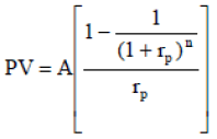(A-1)

Where PV is the fund value at the beginning of retirement (amount to be accumulated during the savings period), A is the amount or pension to be withdrawn every year, n is the number of periods in years that the fund will last during retirement, and rp is the annual rate of return generated by the fund assets during the retirement period. This formula implies that the size of the fund at the end of the retirement period is zero.

A constraint in this formula is that the return >0. Since there is no inflation, the rate of return is real. This formula assumes end-of-period withdrawals. The first pension is withdrawn at the end of the first year. This assumes that the individual retired the previous period and is living off his last annual income.

Estimation of the Savings Rate

Once the total amount to be saved is calculated, the amount needed to be saved in each year to reach this amount is calculated. This is then expressed as a percentage of income. The variables to be considered in calculating the amount to be saved are as follows:

1. Amount to be accumulated.

2. Number of periods in which the savings will take place.

3. Rate of return generated by the funds being saved.

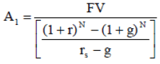
To estimate this figure, the formula to calculate an annuity given a future value is used.

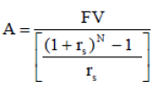(A-2)

Where A is the annuity or amount to be saved or invested each year, FV is the future value or amount accumulated (the fund), N is the number of periods in which the individual is working and saving, and rs is the annual rate of return on the amount being invested during the working period. It is assumed that the first savings amount is deposited at the end of period 1 when the individual receives his annual salary, not earning any return until the following period. To calculate the corresponding savings rate, the resulting annuity is divided by the current annual income.

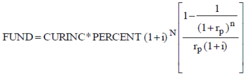
A Combined Equation

Equations (A-1) and (A-2) can be combined into one equation. First, the variables are renamed with more appropriate labels. In equation (A-1), the annuity (A) is the pension sought. Since the pension sought should be a percentage of current income (the replacement rate), these two variables are named PERCENT and CURINC, respectively. PV is the size of the fund needed to support the pension during retirement. This is called FUND. Equation (A-1) becomes:

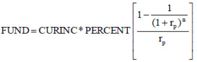(A-3)

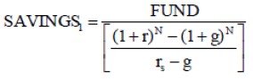
In equation (A-2), the annuity is the amount to be saved each year. We will call it SAVINGS. The FV in this equation corresponds to the fund needed to support the pensions, identified in equation (A-3) as FUND. Equation (A-2) thus, becomes:

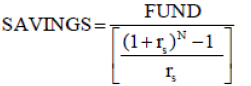(A-4)

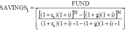
Substituting FUND in equation (A-4) using its equivalence in equation (A-3) results in the following:

(A-5)

Equation (A-5) can be simplified. A simplified equation follows:

(A-6)

If the return during the working period is the same as the return during the retirement period, the equation becomes:

(A-7)

To obtain the percentage of current income that must be saved to reach the fund’s target size, the resulting ANNUAL SAVINGS figure is divided by CURINC.

(A-8)

Where SAVINGS RATE is the percentage of current income that must be saved. PERCENT is still the percentage of current income desired as pension (the replacement rate).

As can be observed, only savings (N) and retirement (n) periods are needed along with a return rate. There is no need to enter dollar amounts. As a first approximation, this simplified equation is very valuable in making gross estimations.

Step Two - Growth in Real Income and No Inflation

An individual who is planning to work for a number of years will see, or at least should expect to see, his real income increase due to promotions attributable to more work experience or enhanced skills. This increase is independent of the rate of inflation. If he keeps saving the percentage indicated by equation (8), his fund’s size will exceed the planned amount. As a result, at retirement, he can decide to withdraw more, or the fund will outlive him, at least in theory. In any case, it would be better to be able to plan for increases in real income. The assumption of zero inflation is still used. The process in developing an equation that combines the savings and withdrawal periods is the same: derive first the equation to calculate the retirement fund including annuities that grow every period in a percentage fashion, followed by the derivation of the equation to estimate the annual savings. A combined equation is derived afterwards

Estimation of the Retirement Fund

Since there is no inflation, the size of the retirement fund just before retirement will be the same given that the pension will not change. Equation (A-3) can still be used.

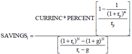
Estimation of the Savings Rate

Once the size of the fund is estimated, a savings amount that increases at the same rate as real income must be estimated in order to keep the savings rate constant. Since this amount will increase each year because of the increase in real income, the formula for growing annuities, also known as graduated payments, is used. In addition to the variables listed before for equation (A- 2), a new variable is now included, the expected growth rate of the annual income. This variable is assigned the letter g. Equation (A-2) becomes:

(A-9)

Where A1 is the first annuity or amount to be saved in the first year, g is the growth rate (in percent) in real income per year, FV is the future value or amount to be accumulated, N is the number of periods or years in which the individual is working and saving, and rs is the annual real rate of return of the amount being saved during the working period. One restriction of this equation is that the rate of return needs to be higher than the growth rate of real income. Renaming the variables, using the same criteria used in renaming equation (A-2), the equation becomes:

(A-10)

Where SAVINGS₁ is the amount to be saved in the first year. This amount is increased by g in the following periods if g, the growth in real income, is different than zero.

A Combined Model

To obtain an equation that incorporates growth in real income, Equation (A-10) is combined with equation (A-3). This results in:

(A-11)

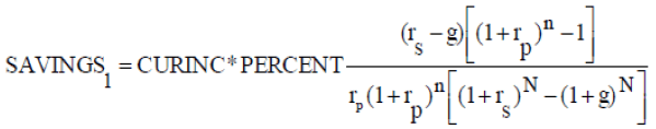
The numerator is the final size of the fund. Further simplification yields:

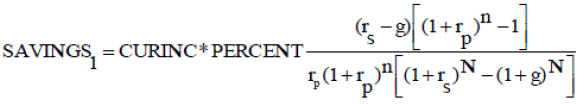(A-12)

Dividing both sides by CURINC and considering that CURINC increases each year by the real growth in income, SAVINGS1 divided by CURINC becomes a constant savings rate. The equation follows:

(A-13)

The value for the growth in real income can be estimated by comparing current entry level salaries for different levels of skills with current salaries at retirement age. i.e.: entry level salaries for college graduates with salaries prior to retirement of college graduates. If the individual using this model is not a college graduate, different entry and exit level salaries can be used to find the annual growth in real income. When the rate of return in the working period (rs) is the same as the rate of return in the retirement period (rp), simplification of the equation doesn’t result in a simpler equation as was the case of equation (A-7)

Step Three - Growth in Real Income and Inflation

Thus far an inflation rate of zero has been assumed. Inflation, though, even in small numbers, is a fact of life. Inflation has an impact on income, expenses and the rates of return. If inflation is factored into the model, the real rates of return and the real growth in income need to be inflated as well. To do this, equations (A-3) and (A-10) are used to calculate the size of the fund (given a desired pension) and to calculate the savings required to build the corresponding fund in the presence of growth in real income. Equation (A-12) could be used, but the process of simplifying the equation would be cumbersome. To adjust real rates for inflation, the Fisher equation, which relates real rates to inflation and nominal rates, is used:

(A-14)

Estimation of the Retirement Fund

After adjusting the rates in equation (A-3) using equation (A-14), the equation used to estimate the size of the required fund becomes:

(A-15)

Where i is the annual expected inflation rate. All the other variables have been defined previously.

Estimation of the Savings Rate

Equation (A-10), which is used to calculate the first savings amount given a fund to be built, becomes the following (after adjusting both the return rate and the growth rate in income for inflation using the Fisher equation (A-14)):

(A-16)

A Combined Equation

Combining equations (A-15) and (A-16) into one and simplifying it results in the following general equation:

(A-17)

This equation does not include the inflation variable. It is the same as equation (A-12), which is used to calculate the savings amount in the presence of growth in real income (step two) with no inflation. The explanation for this result is that the inflation rate affects all rates in the equation (the rates of return and the rate at which real income grows) in the same way. Dividing the annual savings by the current income results in a savings rate which is a percentage of current income as equation (A-18) shows:

(A-18)

The savings rate is constant, thus annual savings will be adjusted as current income increases as a result of inflation and increases in real income. The fact that no inflation rate needs to be estimated simplifies and improves the usability of the model. There is no need to enter an inflation rate, just to enter expected real rates of return and expected growth in real income, which is easier. Compared to changes in nominal income, changes in real income Table lower volatility.

Factoring in Current Accumulated Assets

It is possible that the user of the model already has some retirement savings or has assets that can be used during his retirement to generate additional income. These assets can be added to fund he will build during his working years and will enable him to save less for the same retirement pension amount. In this case, the model should incorporate those assets when calculating the savings amount. These assets will be subject to growth due to a real return and inflation, which will be entered by the user of the model. These assets are identified as the variable CURFUND. The amount of these assets will be subtracted from the estimation of the total fund that needs to be accumulated by retirement.

Using equation (A-1) the following equation is derived:

(A-19)

Where CURFUND is the amount of accumulated savings at the time of using the model and rA is the real return rate of these funds. All the other variables have been defined before. As the model shows, the rate of return of CURFUND can be different. As with the main model, an inflation rate is not part of the model and consequently, there is no need to estimate it. Dividing the savings amount by the current income will result in the savings rate.

References

1. Brown, J., Goda, G., & McGarry, K. (2012). Long-term care insurance demand limited by beliefs about needs, concerns about insurers, and care available from family. Health Affairs, 31(6), 1294-1302.
2. Christman, B.G. (2010). The next retirement hurdle: Why today's employees need more than a savings plan. Benefits Quarterly, 26(2), 30-35.
3. Gist, J.R., Wu, K.B., & Ford, C. Do baby boomers save and, if so, what for? Publication 9906 (Washington D. C., AARP) 1999.  Retrieved from https://assets.aarp.org/rgcenter/econ/9906_do_boomers.pdf
4. Goebel, J.M., & Zivney, T.L. (2014). Prudent savings for lifetime consumption. Journal of Financial Planning, 27(3), 42-51.
5. Gustafson, L.V., Boldt, D.J., & Bird, B.M. (2005). Determining the saving rate necessary for a comfortable retirement. Journal of Personal Finance, 4(3), 62-78.
6. Helman, R., Copeland, C., & VanDerhei, J. (2016). The 2016 retirement confidence survey: Worker confidence stable, retiree confidence continues to increase.  Employee Benefit Research Institute, 397, 1-32.
7. Iglehart, J. (2010). Long-term care legislation at long last? Health Affairs, 29(1), 8-9.
8. Kemper, P., Komisar, H.L., & Alecxih, L. (2005). Long-term care over an uncertain future: what can current retirees expect? Inquiry, 42(4), 335-350.
9. Lew, J.J., Burwell, S., Perez, T. & Colvin, C. (2016). Status of the social security and medicare programs: A summary of the 2016 annual reports. Retrieved from http://www.ssa.gov/oact/TRSUM/tr16summary.pdf
10. Lown, J. (2008). Retirement savings adequacy for the baby boom generation. Journal of Personal Finance. 7(1), 109-134.
11. Lusardi, A., & Mitchell, O.S. (2007). Financial literacy and retirement preparedness: Evidence and implications for financial education. Business Economics, 42(1), 35-44.
12. McManus, G., Sharma, R., & Tezel, A. (2008) Guidelines for retirement net income replacement ratios. The Business Review, 10(2), 40-45.
13. Pfau, W.D. (2011). Safe savings rates: A new approach to retirement planning over the life cycle. Journal of Financial Planning, 24(5), 42-50.
14. Samavati, H., Adilov, N., & Dilts, D.A. (2013). Empirical analysis of the savings rate in the United States. Journal of Management Policy and Practice, 14(2), 46-53.
15. United States. Cong. House. Social Security Administration. Social Security Board of Trustees (2016). Annual Report to Congress. 114th Congress. 2nd Session House Document 114-145. Washington: GPO, 2016. The Library of Congress.
16. Wade, A.H. (2010). Mortality projections for social security programs in the United States. North American Actuarial Journal, 14(3), 113-42.