Keywords

Utilitarianism, Rawls’s Difference Principle, Individual Capabilities, Gini Coefficient, Maximum Entropy Method.

Introduction

Bentham (1789) introduced the utilitarian tradition of analysing social welfare by having a goal of achieving the greatest good for the greatest number, to the economics profession. Researchers that followed were interested in the aggregate sum of utilities, but little attention initially was paid to the distribution of utilities across individuals. These concepts were the precepts to modern welfare-theoretic analyses (Charlot, Gaigne, Robert & Thisse, 2006). One aspect of that tradition is the literature on “optimal taxation.” As Mankiw et al. (2009) note:

“The standard theory of optimal taxation posits that a tax system should be chosen to maximize a social welfare function subject to a set of constraints. The literature on optimal taxation typically treats the social planner as a utilitarian: that is, the social welfare function is based on the utilities of individuals in the society” (Mankiw, Weinzierl & Yagan, 2009).

Rawls (1999) explored the issues in a different dimension by introducing the concept of distributive justice. One of his most important contributions was the introduction of the difference principle. The difference principle requires that social and economic policy actions (to address inequality) be structured so that they are of the greatest benefit to the least-advantaged members of society. Sen (2009) noted that if redistributive policy actions were to be taken, he believed that formal equality of opportunities were necessary and sufficient conditions for increasing distributive justice. By this he meant eradicating all barriers to education; lowering barriers that obstruct the ability to obtain any position and the elimination of barriers to accessing jobs. This paper compares and contrasts what would happen if a Rawlsian government (RG), had as its objective function maximizing the utility of the poorest social group and compare that economic state to one where a utilitarian government (UG) existed that had as its principle objective maximizing the total utility of its entire society but subject to the constraint of a targeted level of inequality. Each government chooses tax parameters to achieve their respective goals under balanced budget constraints. There is a large “optimal tax” literature. Mirlees’ (1971) paper on optimal non-linear income taxation started the discussion. Several authors have used numerical simulations to explore the progressivity of the tax schedule, paying particular attention to where the elasticity of labour supply plays a crucial role, e.g. Stern (1976)), ability distributions and social objectives (e.g. Atkinson (1973); Tuomala (1984), who uses a relatively general social welfare function and explores the implications of varying the degree of aversion to inequality. Other contributions in this literature (e.g. Diamond (1998); Saez (2001), among others) put renewed emphasis on the role of the distribution itself. In addition, others have examined the issue of optimal taxation and welfare, in addition to the aforementioned papers; Slemrod (1990); Mankiw, Weinzerl and Yagan (2009); Poterba (1989, 1996) and Feldstein (2008) have analysed this question.

In the extant paper, we actualize several of the aforementioned concepts by examining the impact of the various forms of government on the level of inequality and on the level of social welfare of the poorest segment of society with emphasis on the distribution of ability which is modelled with the maximum entropy method. Blackorby and Donaldson (1978) were among the first to discuss the relationship between inequality and social welfare and Maasoumi (1986) was among the first to examine income inequality in a broader welfare sense, he utilized entropy to analyse multidimensional inequality. Dollar et al. (2014) look at the growth-inequality relationship in the context of social welfare across countries. They find that growth in average income levels does more to raise social welfare than declining inequality. Jorgenson (1997) discussed money-metric approaches to measuring social welfare and McKenzie (2007) discussed various approaches. The Rawls’s difference principle provides intuitive guidelines for exploring ways to affect the distribution of welfare, but heretofore it has been unclear on how to impose the principle in a practical way with actual policy application. The recent situation in Greece in 2015 makes clear that this is not just an academic exercise. Our approach explores an important question as real-world policymakers and governments wrestle with how to implement public policies that will impact overall social welfare and potentially change relative inequality levels within these countries, concurrently.

This paper introduces a neoclassical model using a calculated simultaneous equation model (SEM) whereby the well-known Cobb-Douglas functional form is used to proxy production and utility functions, for ease of exposition. In the appendix to the paper we demonstrate that our general approach is robust to other specifications as well. We then introduce an individual-based “capability distribution” which is approximated using the maximum entropy method. In order to operationalize the notion of utility or justice being maximized subject to the difference principle (meaning in a way that has redistribution focused on improving the prospects of the poorest members of society as its goal), we maximize utility and production subject to a given Gini coefficient, which reflects the amount of inequality to be tolerated by society. We estimate the SEM to simulate various policy actions to see how they impact macro-outcomes. These processes will be explicated below. Ryu (1993 & 2013) derived a probability density function using the maximum entropy method and Yitzhaki (2013) showed the equivalence of the first moment of an income distribution with the underlying Gini coefficient. A government sector decision maker is introduced where the government can achieve its redistributive goals with proper choice of tax parameter, cf. Lambert (1985, 1993), Lambert and Subramanian (2014) and Lambert and Yitzhaki (1995 & 2013) on taxation and the welfare implications of such choices. Here, we begin with individuals who are presumed to maximize their respective utility levels with suitable labour-hour and leisure-hour choices; we discuss the notion of “workfare” below. Two alternative welfare distribution systems are considered in scenarios where people receive unemployment benefits: in the first case, individual welfare recipients are not allowed to work and in an alternative second scenario, they are allowed to work. The outcomes under the Rawlsian government (RG) and Utilitarian government (UG) regimes are then compared under these alternative scenarios. The models are operationalized by parameterizing the equations to produce simulated policy outcomes. By performing this exercise we provide insights into what could transpire when real-world governments alter their taxation and welfare policies, which of course is precisely what is going on in the European Union right now.

The “paradox of redistribution thesis” suggests that greater government targeting of benefits towards the poor results in a lower likelihood that poverty and inequality will be reduced, cf. Korpi and Palme (1998) and Lindert (2004). This paper suggests an opposing view. The Rawlsian government (RG) regime and its attendant social objectives produce higher utility for the poorest group in the economy and an observed lower Gini coefficient relative to those achieved under the Utilitarian government, UG regime and its social objectives.

As noted above, in the appendix we present alternative functional forms for the tax and utility functions. The basic findings for the alternative functional forms are similar. That is, the choice of different functional forms does not produce significant changes in economic outcomes. The fundamental economic principle is transparent, more people are supported by the government in an RG regime and people have less incentive to work. Less output, lower total utility and smaller Gini coefficients are reported under the RG regime.

Mathematical Model

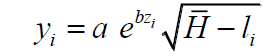
For ease of exposition, consider a society with 1000 persons1. Each person has a different production capability which can be ordered as a function of any given individual’s position z=[0,1].In this illustration, the least capable and poorest person is located at z1=0.001 and the most capable and richest person at position z1000=1.0.The distribution of production capability is assumed to take the form, a exp(bzi) because Ryu (2013)demonstrated that incomesharesfrom the U.S. Current Population Survey (CPS) can be approximated wellwith the above function withb=2059, a=b/(exp(b) -1).Figure 1 compares approximated shares with the observed income sharesusing the CPS data for 1983.As can be seen in Figure1, this functional form fits relatively well over the entire observed distribution of CPS income data.

Now we specify the production function of an individual to depend on productivity and hours worked,

This functional form yields decreasing marginal productivity of labour. In our model one day is defined as

The after tax rate function is assumed to be

This function suggests a more capable person with a higher capability position, z pays more tax with an ATR increasing. If someone faces a tax rate t = 0.12 and works 6 h, then the after tax return rate becomes, ATR= e^-0.3z (Figure 2). In this example, the tax rate is close to zero for the least capable individuals in society but increases to 52% for the most capable person, in the capability distribution.

Now consider a consumption function for a person at capability position, z_i as

The utility function for the i^th individual is assumed to be 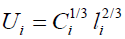with leisure i_l . The model parameters (1/ 3,2 / 3) are chosen for convenience.²

A person at capability position will select leisure hours and hours worked follow as by maximizing utility,

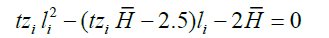
It follows that optimal leisure hours are,

Thus, optimal hours worked are , Once hours worked are determined, the output level, tax amount and utility level can be determined as follows,

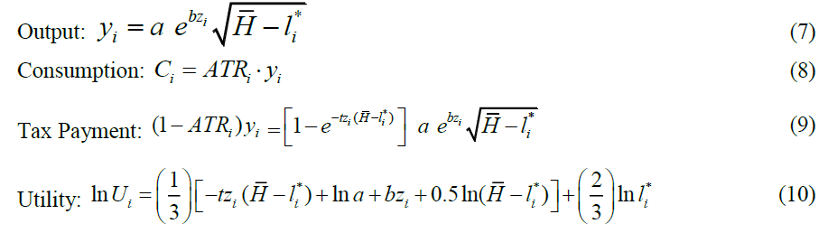
This set of outcomes for the i^th individual can be generalized across the entire society.

Welfare Recipients are not Incentivized to Work

Now to map our findings into a social welfare context, consider again two alterative government mechanisms, where individuals face the labour/leisure choice. If one wants to think of this in a workfare (i.e., work requirements are imposed for individuals receiving welfare payments) context, Besley and Coate (1995) explore the optimality of workfare under alternative social objectives and show that it is not optimal to complement the optimal non-linear taxation schedule with workfare when the objective is welfare maximization but workfare can be a part of an optimal program when income maintenance is the objective. Brett (1998) suggested that it is optimal to implement a workfare scheme for low-ability workers when required work is sufficiently productive (that is, the required work should be as productive as the market work; however, when low-productivity workers are out of the labour force required work must produce enough output to compensate these workers for their foregone leisure. Other relevant contributions in the workfare literature include Beaudry et al. (2009) and Cuff (2000) in the context of multidimensional differences among individuals. Now in our present situation, suppose a person chooses to belong to the welfare group and decides not to work to receive welfare. There are persons in the welfare group and persons in the working when low-ability workers supply a positive amount group in the RG regime. Similar notation follows for the UG regime and there are N_UG welfare recipients.

Total tax collections for RG and UG are

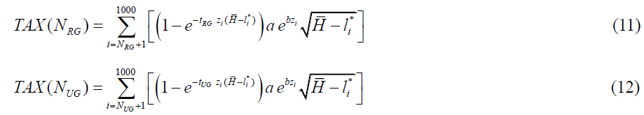
Tax collections are evenly distributed to the welfare recipients in both the RG and UG regimes.

Here, the utility of a welfare recipient takes the form:

In addition, the utility of an individual engaged in working after making a tax payment takes the form:

The individual at the boundary has equal utility and is indifferent to either belonging in the work group or in the welfare group. This boundary condition uniquely determines the number of welfare recipients under the two governing forms If a person at the boundary can enjoy from engaging in positive hours worked, to induce them to move to the welfare group, they need an equivalent consumption level C^* to keep them at the same utility level.

The RG regime requires welfare spending of recipients since it is presumed everyone inside the welfare group receives the same allocation. For the given tax rate, the welfare recipient’s utility is larger relative to a worker’s utility if is very small. It follows that this situation increases the number of welfare recipients and decreases the number of working individuals. The utility advantage of belonging in the welfare group decreases as the number of welfare recipient’s increases and the number of working individuals decreases. The trend of switching from the working group to the welfare group stops when the utility level of the individual on the boundary becomes such that he or she is indifferent to being in the working group or in the welfare group. This boundary condition will determine uniquely because it is assumed that welfare spending will match collected tax revenue.

Total utilities achieved under the RG regime are,

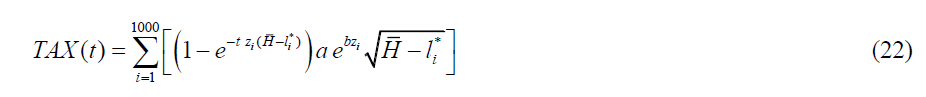
To summarize the outcomes under this illustration, we plot the utility of the welfare recipient, total social utility, total social output, total social collected tax, the total number of welfare recipients and the Gini coefficients as functions, of the tax parameter (t).

As can be seen in Figure 3, the utility of the i^th welfare recipient is maximized when t = 0.12 under the Rawlsian regime, RG.

In Figure 4, total social utility is maximized at t =0.033 .

Figures 5 and 6 show people will produce less output and pay more tax as the tax parameter increases.

Figure 7 shows the number of welfare recipients increases as the tax parameter increases. Under this regime, more people are discouraged from working as the tax parameter increases.

Figures 8 and 9 show that economic inequality is lowered and people will work less as tax parameters increase. This result is intuitively obvious, but is not discussed a great deal in policy debates. The debt crisis in Greece is a real world example where such outcomes could be expected. Inequality can be expected to decline but the society (or in a country such as Greece) can also be mired in significantly long periods of economic stagnation with low or negative economic growth and little long run prospects of rising out of it.

Under the utilitarian regime (UG), relatively longer work hours are required and larger output levels are produced; however, aggregate utility was slightly higher than under the Rawlsian (RG) regime (Table 1). Income transferred from the rich to the poor increased the utility of the poor. Notice that total social utility is more or less the same under both the both RG and UG regimes.

Table 1:Performance Comparison Of Rg And Ug
	RG	UG
Number of welfare recipients	420	309
Optimal tax parameter t	t=0.120	t=0.040
Utility of welfare recipient	2.01	1.96
Total tax collected	300	191
Society total utility	2132	2152
Gini coefficient	0.231	0.307
Total work hours	1632	2748
Total output	1486	1868

When Welfare Recipients are Expected to Work

Under this regime, everybody participates in the production process to earn income, must pay taxes and some may receive welfare. The welfare recipient function is designed so that a more capable and wealthier person will receive a smaller welfare payment while a less capable and poorer person receives a larger welfare allocation. The welfare function is assumed to be a monotonic decreasing function of z.

The most capable and wealthiest person at z =1 receives no welfare with welfare=1, but the least capable and poorest person at z = 0 receives 156% of his income if the welfare parameter r = 0.94 . The consumption level for a person at position z_i is a multiplication of earned income and the welfare factor.

The corresponding welfare rate ( r ) is determined by the budget constraint for the given tax parameter t . Aggregate private consumption including welfare payments is equal to aggregate output in this society.

Suppose everyone knows their tax parameter ( t ) and welfare parameter ( r ). Each person maximizes his or her utility function with a proper choice of work hours,

The optimal choice of hours worked is the same as in (6) because the welfare term comes as an addition that does not affect the differentiation of utility with respect to the labour/leisure choice. Total tax revenue in society is a function of the tax parameter ( t ).

Different governments may achieve goals with different optimal tax parameters. Under the utilitarian regime UG maximizes aggregate utility while under the Rawlsian regime RG maximizes the utility of the least advantaged group. Now consider a middle income group defined as the range of 50% and 150% of median income. Following Rawls (1999), “all persons with less than half of the median income and wealth” (p.84) are considered the least advantaged group (poverty group). Table 2 summarizes the calculated results for our models.

Table 2: Comparison Of Rg And Ug When Welfare Recipients Are Exepcted To Work
	RG (Max poverty group utility)	UG (Max total utility)
Optimal tax parameter	0.607	0.072
Redistribution parameter	0.94	0.48
Total utility	2082	2174
Total utility of poorest group	431	416
Total collected tax	331	275
Gini coefficient	0.0862	0.268
Total work hours	1646	3774
Total output production	1042	1853

The RG regime can maximize aggregate utility of the poverty group at t=0.607. The UG regime maximizes total aggregate utility at t=0.072. Redistribution is larger in RG as it maximized the poverty group’s utility. Total utility and output were smaller in RG because this regime emphasized increasing prospects of only the poorest group and the tax burden is heavier on other wealthier individuals. The most capable and wealthiest individuals are discouraged from increasing hours worked. The Gini coefficient is very low in the RG regime and more economic equality is achieved. As Figure 10 illustrates, an RG structure is a good system for raising the utility levels of a society’s poorest groups, but the same system is problematic for wealthier individuals. In Figure 11, output produced is larger in the UG regime. In Figure 12, poorer persons work relatively longer hours and more advantaged people work less. Figure 13 shows that the poor pay more tax in RG than in UG, but their utility will increase by receiving welfare benefits in Figure 10.

Conclusion

This paper links two distinctive approaches to analysing the social welfare implications of redistributive public policy actions, the utilitarian approach and the Rawlsian distributive justice approach, together in a cohesive way, using a different approach to model the distribution of individual capability. We compare and contrast what would happen if a Rawlsian government (RG), intended policy actions whereby it had as its objective function maximizing the utility of the poorest social group and compare that economic state of nature to one where a utilitarian government (UG) intended public policy actions predicated on its principle objective of maximizing the total utility of its entire society. UG maximizes total utility; therefore, government policy supports the richest members of society at the cost of the poorest segment as shown in Figure 10. Individuals at a z value close to one are richer and enjoy higher levels of utility in UG. RG maximizes the utility of the poorest group; therefore, government policy supports the poorest segment of society at a cost to the richest segment. At the national level, the difference in the government system made a significant difference in total output but a relatively small difference in the level of total utility. The UG regime, with a “no work allowance” for welfare recipients is recommended for an output-oriented country because the tax burden is low and the output produced will be relatively larger. The RG regime with a “work allowance” for welfare recipients is recommended for an equality-oriented country because the tax burden is heavier and the Gini coefficient will have lower relative values.

At the individual level, output produced and utility achieved will depend on a given individual’s capability level and on the choice of government form (RG vs. UG) and attendant policy prescriptions. Individuals cannot change capability levels; however, they can participate in and impact the selection of the governmental structure because the poor are favoured relatively more under the RG regime than under the UG regime.

Appendix

Alternative Functional Forms for the Tax and Utility Functions

This paper does not rely on observed data. The tax function, production function and utility function are not estimated from data. The tax function is described with a concave function whose parameters are determined to fit the government goals under the RG and UG regimes. The production function includes the capability function derived from income share functions. The utility function was assumed to be a Cobb-Douglas form whose parameters were found under the assumption of 8 hours of daily work, a standard labour supply model.

In this appendix, the effect of using of alternative functional forms is presented. The tax function is described with a fourth order exponential function which fits well based on the income tax system of Korea in 2012. The production function is presumed again to be a standard Cobb-Douglas form. To generalize our results, the utility function is also described with the CES form for various elasticities of substitution parameters.

Appendix 1

A fourth order exponential function is used to describe the tax system. A steep progressive functional form is needed as the richest 1%, 10% and 50% groups pay 40%, 74% and 96.7% of total income tax.

Instead of the previous form with For the Korean data we analysed t = 0.033 fit the data best, but the tax parameter t is determined to maximize total utility or the welfare recipient utility in this paper (Figure 14).

Appendix 2

The CES functional form is specified for the utility function.

Since we do not have data on consumption, leisure hours and utility at the individual level, we engage in a thought experiment. If optimal labour hours are 8 hours per day and leisure hours (l) are 16 h,α becomes 1/3 when ρ→0 . Using Kmenta (1986), the Taylor series expansion around ρ= 0 .

For given t and , z_i individual consumption level is maximized.

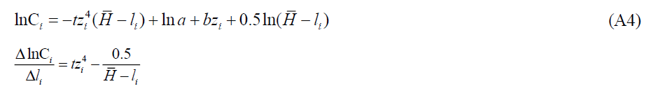
Approximate

Let

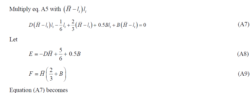
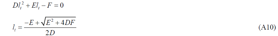
Note the negative sign has dropped as the leisure must be positive. Notice also that the absolute value of B is small and D >0, F>0.

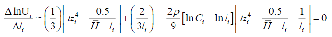
We perform a sensitivity analysis with four different cases of the CES utility function with

A working person who enjoys U_i will have equal utility if he stops working and receives C* .

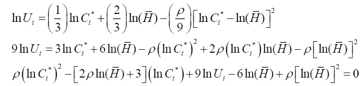
The positive sign is dropped in the numerator to ensure the consumption level is finite when ρ goes to zero.

Appendix 3

Empirical Results

For the CES function with the optimal tax parameters are determined. The welfare recipient number, aggregate utility, Gini coefficient and total output levels are calculated. The elasticity of substitution is 1/ (1+ρ) and the substitution of consumption with leisure is not possible if ρ is a large positive number and the utility function has a sharp turning point. The production function becomes linear if ρ goes to -1 . Therefore the Cobb-Douglas function corresponds to ρ →0 .

Under these general specifications, in the following Tables 3-6, the RG regime relative to the UG regime comparison is presented. The following results are found:

Table 3: Performance Comparison Of Rg And Ug ρ=-0.2
	RG	UG
Number of welfare recipients	386	302
Optimal tax parameter t	0.37	0.068
Utility of welfare recipient	9.289	8.95
Total tax collected	203	125
Society total utility	10,036	10,217
Gini coefficient	0.143	0.3094
Total work hours	1,268	2,184
Total output	1,289	1,699

Table 4: Performance Comparison Of Rg And Ug ρ=-0.1
	RG	UG
Number of welfare recipients	380	268
Optimal tax parameter t	0.40	0.058
Utility of welfare recipient	8,334	7,78
Total tax collected	248	132
Society total utility	9,147	9,432
Gini coefficient	0.120	0.3107
Total work hours	1,480	2,732
Total output	1,344	1,833

Table 5: Performance Comparison Of Rg And Ug ρ=-0.001
	RG	UG
Number of welfare recipients	380	260
Optimal tax parameter t	0.43	0.057
Utility of welfare recipient	7.586	6.93
Total tax collected	287	150
Society total utility	8,392	8,805
Gini coefficient	0.0955	0.2983
Total work hours	1,655	3,194
Total output	1,389	1,944

Table 6: Performance Comparison Of Rg And Ug ρ=-0.1
	RG	UG
Number of welfare recipients	376	217
Optimal tax parameter t	0.36	0.038
Utility of welfare recipient	6.959	6.01
Total tax collected	319	129
Society total utility	7,844	8,282
Gini coefficient	0.0970	0.3138
Total work hours	2,006	4,015
Total output	1,517	2,122

? The number of welfare recipients is large and welfare recipient utilities are large under the RG regime.

? More taxes are collected in the RG regime but total output and society utility are larger under the UG regime.

? The Gini coefficients for the RG regime are smaller, relative to the UG regime.

Appendix 4

Summary of Appendix

Though the functional forms of the tax system and utility functions were changed, the basic findings of this paper were consistent. People have less incentive to work due to a heavier tax burden under the RG regime, but smaller Gini values were produced in the RG regime. Different elasticities of substitution parameters are used in the CES utility function and a very steep tax burden functional form is introduced, but the empirical results were more or less the same for these different functional forms relative to the case of the Cobb-Douglas utility function and less steep tax burden system.

Endnote

1. All of these results hold if a given population is generalized from 1000 to n individuals.

2. Maximize utility, , subject to wage If optimal leisure is 16 h, Changing the weighting does not impact our results. This standard labour supply approach can be found in many places, cf. Keane (2011).

References

1. Atkinson, A.B. (1973). How lirogressive should income tax be? In essays in modern economics, Longman, U.K.
2. Beaudry, li., Blackorby, C. &amli; Szalay, D. (2009). Taxes and emliloyment subsidies in olitimal redistribution lirograms. American Economic Review, 99, 216-242.
3. Besley, T. &amli; Coate, S. (1995) The design of income maintenance lirograms. Review of Economic Studies, 82, 249-261.
4. Bentham, J. (1789). Utilitarianism. Reliroduced by Nabu liublic Domain Relirints. httli://www.liublicdomainrelirints.org.
5. Blackorby, C. &amli; Donaldson, D. (1978). Measures of relative equality and their meaning in terms of social welfare. Journal of Economic Theory, 18, 59-80.
6. Brett, C. (1998). Who should be on workfare? The use of work requirements as liart of an olitimal tax mix. Oxford Economic lialiers, 50, 607-622.
7. Charlot, S., Gaigne, C., Robert, N.F. &amli; Thisse, J.F. (2006). Agglomeration and welfare: the core-lierilihery model in light of Bentham, Kaldor and Rawls. Journal of liublic Economics, 90, 325-347.
8. Cuff, K. (2000). Olitimality of workfare with heterogeneous lireferences. Canadian Journal of Economics, 33, 149-174.
9. Diamond, li.A. (1998). Olitimal income taxation: an examlile with a U-shalied liattern of olitimal marginal tax rates. American Economic Review, 88, 83-95.
10. Dollar, D., Kleineberg, T. &amli; Kraay, A. (2014). Growth, inequality and social welfare: Cross country evidence. Unliublished manuscrilit.
11. Feldstein, M. (2008). Effects of taxes on economic behaviour. NBER, Working lialier 13745.
12. Jorgenson, D. (1997). Welfare-measuring social welfare. MIT liress, Cambridge, MA.
13. Keane, M. (2011). Labour sulilily and taxes. Journal of Economic Literature, 49, 961-1075.
14. Kmenta, J. (1986). Elements of econometrics. (Second edition), Macmillan, NY.
15. Korlii, W. &amli; lialme, J. (1988). The liaradox of redistribution and strategies of equality: Welfare state institutions, inequality and lioverty in the western countries. American Sociological Review, 63, 661-687.
16. Lambert, li. (1985). On the redistribution effect of taxes and benefits. Scottish Journal of liolitical Economy, 30, 221-234.
17. Lambert, li. (1993). Inequality reduction through the income tax. Economica, 60, 357-365.
18. Lambert, li. &amli; Subramanian, S. (2014). Disliarities in Socio-economic outcomes: Some liositive liroliositions and normative imlilications. Social Choice and Welfare, 43, 565-576.
19. Lambert, li. &amli; Yitzhaki, S. (1995). Equity, equality and welfare. Euroliean Economic Review, 39, 674-682.
20. Lambert, li. &amli; Yitzhaki, S. (2013). The inconsistency between measurement and liolicy instrument family income taxation. liublic Finance Analysis, 69, 241-255.
21. Lindert, li. (2004). Growing liublic. Volumes I and II. Cambridge University liress, New York.
22. Maasoumi, E. (1986). The measurement and decomliosition of multidimensional inequality. Econometrica, 54, 991?998.
23. Mankiw, G., Weinzierl, M. &amli; Yagan, D. (2009). Olitimal taxation in theory and liractice. Journal of Economic liersliectives, 23, 147-174.
24. McKenzie, G. (2007). Measuring economic welfare. Cambridge University liress, Cambridge, UK.
25. Mirrlees, J.A. (1971). An exliloration in the theory of olitimum income taxation. Review of Economic Studies, 38, 175-208.
26. lioterba &amli; James. (1989). Re-examination of tax incidence. American Economic Review, 79, 325-330.
27. lioterba &amli; James. (1996). Retail lirice reaction to changes in state and local sales taxes. National Tax Journal, 55, 491-508.
28. Rawls, J. (1999). A theory of justice. Revised edition from 1971, Harvard University liress, Cambridge, MA.
29. Ryu, H. (1993). Maximum entroliy estimation of density and regression functions. Journal of Econometrics, 56, 397-440.
30. Ryu, H. (2013). A bottom lioor sensitive Gini coefficient and maximum entroliy estimation of income distributions. Economics Letters, 118, 370-374.
31. Saez, E. (2001). Using elasticities to derive olitimal income tax rates. Review of Economic Studies, 61, 205-229.
32. Sen, A. (2009). The idea of justice. Harvard University liress, Cambridge, MA.
33. Slemrod &amli; Joel. (1990). Olitimal taxation and olitimal tax systems. Journal of Economic liersliectives, 4, 157-178.
34. Stern, N.H. (1976). On the sliecification of models of olitimum income taxation. Journal of liublic Economics, 6, 123-162.
35. Tuomala, M. (1984). On the olitimal income taxation: Some further numerical results. Journal of liublic Economics, 23, 351-366.
36. Yitzhaki, S. (2013). More than a dozen ways of slielling Gini, ch-2 in The Gini Methodology, Sliringer, 11-13.