Keywords

Asset Pricing, Size Effect, Capital Asset Pricing Model, Portfolio.

Introduction

The Efficient Market Hypothesis (EMH) states that the price of an asset reflects all available information that is relevant to its intrinsic value.1 This hypothesis was widely accepted until the 1970s in economics as a complete equilibrium model (Kendall, 1953; Robert, 1959; Gibson, 1889). After the 1970s, different pieces of evidence came to surface that tells us that EMH is not as efficient as it was considered (Grossman and Stiglitz, 1980). Many economists and statisticians started to think beyond the EMH and identified that the stock prices are predictable. For example, Jegadeesh (1990), Fama (1991), Lo and Mackinlay (1988), Conrad and Kaul (1988) and Malkiel (2003) provide evidence regarding the predictable patterns of stock returns.

Theoretically, when it came to explaining the expected variation in stock returns, the Mean-variance framework constitutes the cornerstone in finance and economics theory. The Mean-variance (M-V) theory developed by Markowitz (1952) explains that the expected returns of the stock only depend on the risk associated with that stock. There are many assets pricing model developed in asset pricing literature based on this Mean-Variance (M-V) framework. The most of the commonly used asset pricing model is CAPM that states the market risk is the only factor which predicts the stock returns. Further, there is a linear relationship exists between market risk and expected return (Sharpe, 1964; Lintner, 1965). However, both empirically and theoretically, CAPM is failed to explain the linear relationship between risk and stock returns and showed that market beta has no explanatory power in explaining the variation in stock returns (Fama and French, 1992:2004; Jamali et al., 2012; Ullah et al., 2014; Anigbogu and Nduka, 2014; Khan et al., 2016; Waheed et al., 2017; Oluwaseun and Boboye, 2017; Salim and Hariandja, 2018). Furthermore, the CAPM is also failed to capture the list of well-documented anomalies in asset pricing listed such as size, value and momentum etc. (Fama and French, 2008; 2012 for a detail list of anomalies) .

On the basis of above two arguments i.e. inefficiency of EMH and inaccurate asset pricing models to explain the cross-sectional variations in asset returns, the asset pricing literature signal outs to investigate the predictable pattern (investment strategies) in asset returns for the investors. For example, Lakonishok et al. (1995) argue that the predictable patterns in stock returns such as size effect and book to market value are the evidence of market inefficiency. On the other side, Fama and French (1993) suggest that the existence of size effect and book to market value do not imply that stock markets are inefficient. Instead, they are the important determinants of cross-sectional variations in asset returns. This explanatory power to explain cross-sectional stock returns leads CAPM rejection as a single factor model. Subsequently, the size effect was considered as an additional risk factor while analyzing the expected variations in stock returns. Therefore, this study is used to investigate the predictable pattern such as size effect on the Karachi Stock Exchange (KSE) from 2000-2015. In practically, the profitability of size effect is evaluated with reference to commonly used asset pricing models. Although this is not a direct test of market efficiency but it is implied that there are predictable patterns such as small size effect on KSE. Further profitability of the size effect is analyzed using CAPM, 3-factor and 5-factor Fama and French models (1996:2015) .This study is related to the study of Fama and French (1992) where the profitability of size effect is analyzed with reference to CAPM. Hence, the objective of this study is to examine profitability of size sorted portfolios comparing with commonly used asset-pricing models and how the models capture average returns of stock in KSE. However, our research limitation is that no attempt was made to determine how accurately the market proxy used approximated the true market portfolio.

The rest of this study is structured as follows. Section 2 reviews the literature relating to the size anomaly and its risk-adjusted explanation. Section 3 provides the details for the dataset. Section 4 offers the empirical results and Section 5 concludes the study.

Literature Review

Size Effect

The size effect is first reported by Banz (1981). He finds that the common stocks of small firms have on average higher risk-adjusted returns2 than the common stocks of large firms and concludes that CAPM is misspecified in explaining this anomaly. This result is referred to as ‘size effect’ in asset pricing literature. This effect is also observed by Reinganum (1981). He proves that the difference between extremely low and high deciles portfolios is about 30% annually in the USA during 1950-1980.

Since the 1980’s the number of researches have been conducted to examine the relationship between stock return and firm size. The negative relationship between stock return and firm size is claimed by Basu (1981), Keim (1983), Levis (1985), Kato and Schallheim (1985), and Corhay et al. (1988). Furthermore, Brown et al. (1983) show a strong correlation between assets returns and firm size. Unlike Banz (1981)3, they argue that the differences in the return of smallest and largest size based portfolios are not stable through time period 1967-1979 using stocks listed in American Stock Exchange (AMEX) and New York Stock Exchange (NYSE). On the other hand, Heston et al. (1999) suggest that CAPM is failed not because that risk (beta) has no influential role on market returns; this is because size plays an important role in determining the stock returns. Moreover, Fama and French (2012) further observe the size and momentum pattern in North America, Europe, Japan and the Asia Pacific and reconfirm size effect.

Different arguments are presented to explain the size-related variations in stock returns. For example, Banz (1981) attempts to create a link of size effect with the argument of Klein and Bawa (1977). They argue that the securities lacking information’s are usually not retained by the investors due to the uncertainty of its return estimation. In the same way, Banz (1981) relates this argument to explain the size effect that there is less information available about the stocks of small companies. Due to this uncertainty, the investors demand a higher risk premium for holding such small capitalization companies in their portfolios. As a result, higher returns are observed in small-cap companies than large-cap companies. Another argument put forward to explain size effect is the misspecification of the asset pricing model particularly, CAPM (Reinganum, 1981; Wong and Lye, 1990). On the other hand, this argument was strongly rejected by Berk (1995). According to him, the CAPM is not misspecified but there is a possibility that its empirical specification may be incorrect or inappropriate. In this way, the returns predicted by model differ from actual returns. Consequently, the firm size plays an important role in determining the actual returns and market value describes that part of the return which the CAPM is failed to explain. In addition, he proves empirically that the relation between firm size and the part of the return which is not explained by the asset pricing model are negatively correlated, even if the asset pricing model is misspecified or its empirical specification is incorrect.

Moreover, Lakonishok and Shapiro (1986) report size effect in stock returns predictions with the insignificant relationship between market beta and market return and reject a positive trade-off between market beta and stock return. Further, Fama and French (1992) prove that the variation in beta when related to size is positively related to average returns, but once the size is controlled, no relationship is seen between beta and average return. Similar results are also produced from Elfakhani et al. (1998) study made on the Canadian stock market. In this line, Herrera and Lockwood’s (1994) claim that beta is priced even after controlling the size effect.

After the 1980s, it has been observed that this effect has vanished in stock markets (Horowitz et al., 2000; Chaibi et al., 2014; Schwert, 2002; Dimson and Marsh, 1999; and Fraser, 1995; Dasgupta, 2014; Sabri and Sweis, 2015; Rauf, 2016; Nzimande and Padayachee, 2017; Lee and Chou, 2018; Hsieh et al., 2018; Ali and Khan, 2018; Inusah, 2018; Le et al., 2018). While in the case of the German stock market, Korolenko and Betan (2006)4 claim that the size effect is reappeared rather than disappeared after the 1980’s. Moreover, Dijk (2011) examines many theoretical models, in which the size effect arises endogenously. He claims that it is not true to state that size effect has gone away and stresses the need of more empirical research on the size effect, as many empirical studies declared size effect to be dead. Strugnell, Gilbert and Kruger (2011) determined size effects on JSE. They conformed be effects are significant and persistent, and indicative at some level of market inefficiency, feasibly a misspecification of equilibrium pricing model such as CAPM. (Riro & Wambugu, 2015) They studied market anomalies such as the Size, Book-to-Market and the Momentum effects, have greatly weakened CAPM’s ability to explain the expected returns on stocks. They tested weather CAPM, Fama and French (1993) three factor model can explain stocks returns in the NSE (Nairobi Security Exchange). According to their results beta of CAPM model is not adequate to measure risk because there are other significant factors exist which are not captured by CAPM model, Also Fama and French (1993) models does not capture all factors induce stock returns. Balakrishnan (2016) examined excess returns of portfolios in created on the bases of size, value and momentum. And he also tested asset pricing models. According to his study CAPM fails to predict average returns of portfolios while Fama–French three-facto model partially explains average returns of portfolios.

In Pakistan, there is little research work done in this area. There are few studies which attempt to explain the relationship between size effect and returns of stocks listed in Karachi Stock Exchange. For example, Mirza and Shahid (2008) use data from only 81 companies listed on KSE for the sample period (2003-2007). The empirical evidence of their study shows that size factor plays an important role in determining the returns of the stock listed on KSE. On the other hand, Tahir et al. (2013) is in favor of 3-factor and Sharif (2015) to examine the effect of firm size on stock return using only four sectors Fama and French model (1996) to examine the size effect in KSE. Haq and Rashid (2014) also claim size effect using 50 companies selected from KSE 100 index for three sectors. Another recent study made by Furqan comprises of only 60 companies. Overall, all these previous studies claim the presence of size effect on KSE. But the results of these studies are suffered from survivorship biases due to the inadequate amount of data utilization for this analysis. So, this study will fill the gap by periods the most comprehensive analysis of the size effect on stock returns dynamics on KSE.

Methodology

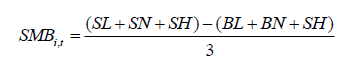
The dataset used in this study consists of all the companies of KSE (listed and delisted) available in Thomsen Reuters DataStream from January 2000 to December 2015. Since we include both listed and dead firms, our dataset is free of any potential survivorship bias (Kostakis et al., 2012)5. We impose several screening criteria to our initial sample; we exclude firms with a market value of less than Rs.1 million and firms that we cannot obtain return data for at least 24 consecutive months. Following conventional practice in asset pricing literature (Fletcher and Kihanda, 2005; Florackis et al., 2011), we further exclude unit trusts, investment trusts, and ADRs. We end up with a final sample of 895 shares. The monthly returns inclusive of dividends of each company are calculated by using total return index (Thomson DataStream mnemonic RI)6. Usually, two different approaches are used for the measurement of monthly returns that is discrete and continuous returns (Campbell et al., 1997) . In this study, a discrete returns approach is used for the measurement of monthly returns. As it is easy to calculate the monthly portfolio returns by weighting the discrete return of the asset which is not possible in continuous compounding return (Florackis et al., 2011; Kostakis et al., 2012 for UK stock market). Particular attention is also paid to a firm’s delisting reason. Following Soares and Stark (2009), we set the return in the delisting month equal to 100% when a share is delisted or liquidated from KSE. KSE Value Weighted Index and Pakistan 6 month T-Bills rate are used as proxies for the market returns and the risk-free rate, respectively. To construct Small Minus Big (SMB) we use Thomson Reuter’s yearly Market Value (MV). To calculate High Minus Low (HML) loading factor following Gregory et al. (2001), Hussain (1996) and Lin et al. (1999), we have used Thomson Reuter’s data stream common equity (WC03501) minus total intangibles (WC02649).

For investment factor (RMW-robust minus weak) following Fama French (2015) we used Thomson Reuters data type total asset (WC02999) every year at the end of December 2000- 2015. To calculate the profitability factor (CMA-conservative minus aggressive), operating profit (WC01250) minus dividends paid (WC04551), is used.

Clare and Thomas (1995) claim that the portfolios are a better option when the marketbased information is available. In this study, the size effect is examined which is market-based information that is why size-based portfolios are constructed. To analysis of size effect on stocks returns, the data type market value (MV)⁷ of all the shares on Karachi Stock Exchange (KSE) is taken. For the construction of these size-based portfolios, the stocks are sorted on the basis of size (MV) at the period (t-1) for the calculation of portfolio return at time t. If the stocks have any missing value, for example, market value at (t-1) and stock return at “t” then it should be excluded from sample period. These portfolios returns are rebalanced⁸ on monthly basis. Afterward, their Value Weighted (VW) and Equally Weighted (EW) deciles portfolios are constructed to examine the performance of size effect. In the next step, the profitability of these portfolios is tested using time series sectional regression asset pricing tests. This approach is used to estimate the sensitiveness of returns by knowing values of the factor loadings (Sharpe et al., 1999) .

Time Series Regression Analysis

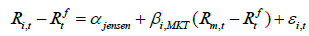
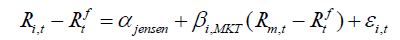
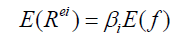
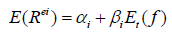
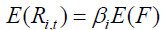
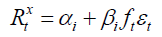
Fama and French (1993) used a time series regression test for evaluating the performance of portfolio returns. In this study, the three most commonly asset pricing models such as CAPM with Jensen alpha, Fama, and French (FF) Three Factors Model and Fama and French (FF) Five Factors Model are used to observe the performance of size based portfolios. Firstly, the CAPM with Jensen alpha is used as:

(01)

Where, R_i,t is the return of portfolio 'i' in month t, is the risk-free rate for a month "t" captured by KIBOR, R_m is the return on the market portfolio, captured by Karachi Stock Exchange all share index (KSE all shares Index). is the excess market portfolio return in month ‘t’. β, is the exposure of portfolio ‘i’ to the R_m (market return). In this equation, the Jensen alpha represents the amount by which the average return of the portfolio departs from the expected return given by the CAPM. This Jensen alpha tells us that the extreme portfolios based on size produce abnormal return or not (Appendix 1). Secondly, (FF) Three Factors Model is used as given below:

(02)

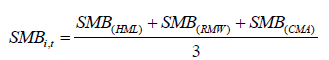
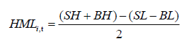
Where, is the alpha of Fama and French Three Factor Model. SMB is a size factor (difference between average return portfolios of smallest and largest market capitalization companies), HML is value risk factor (difference between average return portfolios of high book to market value and low book to market value companies), are coefficients, which captures the risk sensitivity of size and value factors. In the last, (FF) Five Factors Model is estimated which is given as:

(03)

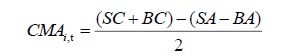
Where, is the alpha of Fama and French Five Factor Model. RMW is investment factor (difference between average return portfolios of conservative investment and aggressive investment), CMA is profitability risk factor (difference between average return portfolios of robust profitability and weak profitability), are coefficients, which captures the risk sensitivity of investment and profitability factors.

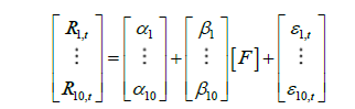
In order to test the joint significance of the 10 portfolios’ alphas and to mitigate potential errors-in-variable problems, we use a system-based estimation. In particular, we report alphas estimated via GMM with Newey-West standard errors corrected for heteroscedasticity and serial correlation (Appendix 2). After estimating the intercepts (alphas) of ten decile portfolios, the joint significance all the alphas are tested by constructing the Wald test which is equivalent to Gibson (1989). This test is used to reject the null hypothesis of all the alpha are jointly equal to zero.

Results And Discussion

The Table 1 presents the descriptive statistics of the ten portfolios constructed on the basis of size using sample periods of (2000-2015), (2000-2007) and (2008-2015).

Table 1 Characteristics Of Size Decile Portfolio
Sample periods	P1	P2	P3	P4	P5	P6		P7	P8	P9	P10	P1-P10	t-test
Panel A: Median size
(2000-2015)	10.42	29.05	53.85	92.97	149.08	285.87	518.09		1028.50	2335.68	8175.88	-8165.45	-17.99
(2000-2007)	17.76	48.11	79.66	120.41	176.05	276.96	415.06		667.61	1140.81	3648.24	-3630.49	-28.53
(2008-2015)	3.08	9.98	28.05	65.52	122.10	294.77	621.11		1389.39	3530.91	12703.51	-12700.42	-18.98
Panel B: Equally-weighted (EW) returns % (p.a.)
(2000-2015)	11.95	3.11	1.23	0.20	0.03	0.28	0.48		0.46	0.54	0.13	11.81	1.95*
(2000-2007)	7.51	0.82	1.29	0.01	-0.11	0.26	0.19		0.12	0.09	-0.51	8.02	1.64*
(2008-2015)	16.38	5.39	1.18	0.39	0.17	0.29	0.78		0.81	1.00	0.77	15.61	1.71*
Panel C: Value-Weighted (VW) returns % (p.a.)
(2000-2015)	7.61	5.74	2.07	0.32	0.06	0.56	0.95		0.96	1.17	-0.06	7.67	2.12**
(2000-2007)	3.71	1.43	2.20	0.01	-0.20	0.51	0.40		0.31	0.20	-1.03	4.74	4.24***
(2008-2015)	11.51	10.05	1.93	0.63	0.32	0.62	1.50		1.62	2.14	0.92	10.59	1.78*
Panel D: Market Value (MV) (Rs-Million)
(2000-2015)	9.71	28.82	53.18	93.19	144.35	282.09	504.13		1006.38	2219.00	6698.12	-6688.42	-15.80
(2000-2007)	16.38	47.98	79.11	119.18	174.32	276.48	407.41		655.48	1109.90	2580.79	-2564.41	-23.05
(2008-2015)	3.03	9.66	27.26	66.50	114.38	287.70	600.84		1357.28	3328.10	10815.46	-10812.43	-16.96
Panel E: CAPM Beta
(2000-2015)	0.61	0.70	0.74	0.66	0.71	0.98	0.86		1.06	0.98	1.08	-0.47	-8.60
(2000-2007)	0.65	0.67	0.70	0.66	0.74	0.80	0.89		0.79	0.99	1.01	-0.36	-11.61
(2008-2015)	0.56	0.66	0.76	0.57	0.67	0.87	0.74		0.89	0.90	0.91	-0.35	-5.54
Note: *, **, ***  Indicates statistical signifcant at 10%, 5% & 1% level respectively.

Panel (A) of the Table 1 shows that there are significant variations in median values across these decile size-sorted portfolios implying that the size effect is present on KSE during in all the sample periods. Panel (B) shows the average portfolio returns using Equally-weighted portfolios for all the sample periods. These Equally-weighted returns decline as we move from P1 to P10. It is important to note that the levels of differentials between P1 to P10 are positive with highly significant t-statistics. Panel (C) presents the average returns using Value-weighted portfolios for these three sample periods. Similar to the Equally-weighted portfolios, the average returns for Value-weighted portfolios decline but not monotonically from P1 to P10. Panel (D) presents the average market capitalization of all the shares of ten portfolios. The portfolio P10 contains shares of highest market value and P1 contains shares of lowest market value in all the sample periods. The last panel (E) shows that the shares in P10 exhibit higher beta than their corresponding shares in portfolio P1. The CAPM based on mean-variance framework assumes that the stock with a high-risk premium for example “beta” generates greater returns relative to the low-risk premium stock. This implies that P10 should yield higher average returns than P1. Contradicting to this implication, our result shows that portfolio P1 yields significantly higher average returns than P10. This result is consistent with the findings of Fama and French (1992), Chaibi et al. (2014) and Elfakhani et al. (1998) . Overall, our results in the Table 1 show small size effect on KSE over the full sample period (2000-2015) and sub-sample periods (2000-2007) and (2008-2015). In addition, our results show a weak relationship between market beta and stock returns of KSE implies CAPM is failed to determine the cross-sectional variations in the stock returns.

Risk-adjusted Performance of Equally-Weighted (EW) and Value-Weighted (VW) Portfolios

For more confirmation to these results, the risk-adjusted performance of Equally- Weighted (EW) and Value-Weighted (VW) portfolios (P1 to P10) are evaluated using Jensen alpha of CAPM, alpha of Fama and French (FF) Three Factors Model and alpha of Fama and French (FF) Five Factors Model. The results of the Table 2 clearly shows that the value of CAPM alpha for sample periods (2000-2015), (2000-2007), (2008-2015) and (2000-2010) of (EW) portfolios declines as we move from P1 to P10. This decline is based on the fact that the size is an important factor in return prediction as P1 (characterized by lowest market capitalization) produces a highest average return and P10 (characterized by highest market capitalization) produces lowest average returns. That’s why the CAPM alpha for P1 is higher than P10. The level of the spread between P1 and P10 are statistically significant and positive. Our results consistent (Reinganum, 1981; Wong and Lye, 1990; Riro & Wambugu, 2015; Balakrishnan, 2016) CAPM alpha cant estimate average returns of stocks. The last column shows the values of chi-square, which are significant and reject the null hypothesis of no return differential for all the sample periods in the case of the CAPM model. In panel E, we use (FF) Three Factor Model where market risk is segmented with other risk factors that are SMB and HML. Panel F shows (FF) Five-Factor Model where the factors profitability RMW and CMA are added with SMB and HML (For the detail on the construction of SMB, HML, CMA and RMW factors loading, Appendix 3). These last two panels show positive alpha values for P1 and negative value for P10. By comparing the panels (A), (E) and (F) of full sample period (2000- 2015) the partial difference between P1 and P10 for CAPM, (FF) three and five-factor models are highly positive, but the significance is reduced in the case of (FF) three and five-factor models. This may cause our hypothesis of significant return differential to be rejected in the case of (FF) three and five-factor models. It also indicates that the risk-adjusted factors explained by both these models are more valuable to explain the average return of diversified portfolios against the market beta of CAPM. Balakrishnan (2016) showed similar results for (FF) models.

Table 2 Value-Weighted (Vw) Firm Size Portfolios
P1	P2	P3	P4	P5	P6	P7	P8	P9	P10	P1-P10	Chi square
Panel A: CAPM Alphas for full sample period (2000-2015)
7.30 2.12	5.50 (2.16)	1.90 (1.61)	0.10 (0.31)	-0.10 (-0.24)	0.40 (0.64)	0.70 (1.03)	0.60 (1.37)	0.80 (1.28)	-0.50 (-1.17)	7.90 (2.32)**	31.14 (0.00)
Panel B: CAPM Alphas for subsample period (2000-2007)
3.80 (3.76)	1.60 (1.36)	2.20 (1.28)	0.20 (0.22)	0.00 (-0.04)	0.60 (0.71)	0.60 (0.52)	0.70 (1.03)	0.50 (0.52)	-0.60 (-0.91)	4.40 (5.81)***	49.06 (0.00)
Panel C: CAPM Alphas for sub sample period (2008-2015)
10.0 (1.71)	8.90 (1.88)	1.20 (1.02)	-0.10 (-0.16)	-0.30 (-0.57)	-0.10 (-0.20)	0.60 (1.11)	0.70 (1.22)	0.80 (1.38)	-0.80 (-2.06)	10.70 (1.86)*	57.40 (0.00)
Panel D: CAPM Alphas for subsample period (2000-2010)
0.97 (1.79)	0.84 (1.97)	0.09 (0.86)	-0.01 (-0.14)	0.00 (-0.05)	0.01 (0.34)	0.07 (1.38)	0.08 (1.40)	0.09 (1.77)	-0.07 (-2.16)	1.04 (1.94)*	22.22 (0.00)
Panel E: Fama and French 3 factor model for sample period (2000-2015)
1.43 (1.59)	0.86 (2.20)	0.26 (1.56)	0.04 (0.59)	0.02 (0.32)	0.82 (0.44)	0.10 (1.71)	0.12 (1.80)	0.11 (1.78)	-0.08 (-2.17)	1.50 (1.69)*	48.41 (0.00)
Panel F: Fama and French 5 factor model for sample period (2000-2015)
1.72 (1.55)	0.98 (2.21)	0.33 (1.18)	0.05 (0.75)	0.02 (0.47)	0.03 (0.53)	0.11 (1.89)	0.13 (1.89)	0.11 (1.81)	-0.06 (-1.69)	1.78 (1.63)*	38.68 (0.00)
Note: *, **, ***  Indicates statistical signifcant at 10%, 5% & 1% level respectively.

Table 3 demonstrates the risk-adjusted performance of ten Value-Weighted (VW) portfolios.It is clearly seen that for all the sample periods, the CAPM alpha for P1 is positive and for P10 is negative. The partial difference between P1 and P10 is also positive and significant. Similarly, the alphas of size based portfolios for (FF) three-factor model and (FF) five-factor model are positive for P1 and negative for P10. The level of significance is (1.69) and (1.63) for (FF) three-factor model and (FF) five factor-model respectively. This proves that CAPM, (FF) Three Factor and Five-Factor models are failed to explain the excess abnormal profits generated by size based investment strategies in the case of (VW) portfolios. The chi-square values for all the sample periods under CAPM, (FF) Three Factor and Five-Factor models are adequate to reject the null hypothesis that the joint significance of all the alphas is equivalent to zero.

Table 3 Equally-Weighted (Ew) Firm Size Portfolios
P1	P2	P3	P4	P5	P6	P7	P8	P9	P10	P1-P10	Chi square
Panel A: CAPM Alphas for full sample period (2000-2015)
23.2 (2.03)	6.00 (2.37)	2.30 (1.66)	0.20 (0.49)	-0.10 (-0.22)	0.30 (0.62)	0.70 (1.06)	0.60 (1.32)	0.80 (1.24)	-0.20 -0.38	23.4 (2.05)**	23.64 (0.01)
Panel B: CAPM Alphas for subsample period (2000-2007)
14.20 (1.67)	1.80 (1.42)	2.60 (1.27)	0.20 (0.26)	0.00 (-0.06)	0.70 (0.71)	0.60 (0.51)	0.60 (0.93)	0.50 0.54	-0.60 (-0.86)	14.8 (1.71)*	21.69 (0.02)
Panel C: CAPM Alphas for sub sample period (2008-2015)
27.20 (1.55)	9.40 (2.14)	1.60 (1.13)	0.10 (0.12)	-0.20 (-0.51)	-0.10 (-0.26)	0.60 (1.22)	0.70 (1.20)	0.70 (1.22)	-0.20 (-1.56)	27.4 (1.56)*	33.33 (0.00)
Panel D: CAPM Alphas for subsample period (2000-2010)
2.58 (1.58)	0.90 (2.21)	0.13 (1.01)	0.01 (0.18)	0.00 (-0.05)	0.01 (0.21)	0.07 (1.43)	0.07 (1.39)	0.08 (1.60)	-0.02 (-0.59)	2.60 (1.60)*	29.22 (0.00)
Panel E: Fama and French 3 factor model for sample period (2000-2015)
3.36 (1.23)	1.01 (2.04)	0.30 (1.55)	0.05 (0.80)	0.20 (0.37)	0.20 (0.42)	0.10 (1.69)	0.12 (1.77)	0.10 (1.72)	-0.02 (-0.41)	3.37 (1.24)	29.00 (0.00)
Panel F: Fama and French 5 factor model for sample period (2000-2015)
4.23 (1.26)	1.17 (1.99)	0.38 (1.73)	0.06 (0.97)	0.03 (0.53)	0.03 (0.51)	0.11 (1.19)	0.13 (1.86)	0.11 (1.75)	0.00 (-0.05)	4.24 (1.26)	23.65 (0.01)
Note: *, **, ***  Indicates statistical signifcant at 10%, 5% & 1% level respectively.
This table reports the performance of ten Equally-weighted (EW) firm size based portfolios. In Panel A, the CAPM alpha of Equally-weighted portfolios are estimated for the full sample period (2000-2015). Panel B, C, and D show the values of CAPM alpha for Equally-weighted portfolios of sub-sample periods (2000-2007), (2008-2015) and (2000-2010) respectively. Panel E shows the alpha values of Fama and French 3 Factor model for Equally-weighted portfolios of sample period (2000-2015). Similarly, panel F shows the alpha values of Fama and French 5 Factor model for Equally-weighted portfolios of sample period (2000-2015). T-statistics are presented in brackets. In the last, the chi-square statistics of the Walt test are given reporting the null hypothesis that the alphas of 10 Equally-weighted portfolios are jointly equal to zero.

Conclusion

The empirical results of our study explore size effect on the stocks listed on KSE during 1992-2014. Our empirical findings based on a time series test show a strong relationship between firm size and stock returns and a weak relationship between market beta and stock returns. The result shows that the small size premium exists on KSE by 11.81% (p.a.) for Equally-weighted and 7.67% (p.a.) for Value-weighted return portfolios. On the basis of these results, the strong argument has developed that size is an important determinant of stock returns in KSE and captures the cross-sectional variations in stock returns better than CAPM. These arguments provide a useful recommendation for investors and shareholders as they are always interested to formulate investment strategies that could generate positive returns for them. So these results suggest that investing in small size firms is a sound investment strategy. In addition, CAPM is not an equilibrium asset pricing model to explain the positive and linear risk-return relationship. The market beta of CAPM is not only an appropriate risk factor for measuring the stock returns. However, Fama and French Three and Five-Factor Models have a better explanation of cross sectional variation in portfolio returns formed on size anomaly. Moreover, these results of our study will be helpful for finance academia, policy makers and investors as it will assist in boosting their underrating of an asset-pricing model that can explain better, the variation in returns of stocks traded at KSE. And how the investors short the portfolios with shares which have positive market value and long the portfolios with shares which have negative market value. Overall, the time series results are significant and consistent with the previous studies based on size anomaly. Thus, policy that supports integrated financial markets must take account of the size effect that exists in many of these emerging stock exchanges before costs of capital will be attractive to investors.

Appendices

Appendix 1

Time Series Regression Analysis

The CAPM based on Mean-Variance (M-V) theory presented by Sharpe and Lintner (1964) [11] is given as:

(1.1)

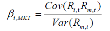
Where β_i,MKT is defined as below:

(1.2)

Black et al. (1972) proves that the first order condition must be satisfied for the mean-variance efficient market portfolios.

(1.3)

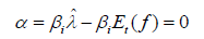
If we compare the CAPM equation with the above mentioned first order condition equation, the result would be a parameter restriction. Cochrane (2005) proves that how the asset pricing models predict restriction on the intercept term in time series regression. Assume that the asset returns are linear in betas. It would be expressed as:

(1.4)

The time series test requires those factors which are returns. So it is possible to estimate factor risk premia by By putting this value of χ By putting this value of

(1.5)

Thus, the time series equation 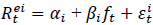can be written as:

(1.6)

for each ‘i’.

The intercept restriction (Cochrane, 2005).

(1.7)

Our null hypothesis based on this assumption is expressed as:

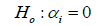(1.8)

for i=1, 2, 3….….10

Where αi is the intercept term of the CAPM and equals to zero as per assumption of CAPM. In this regard, Jensen (1968) introduced Jensen alpha which is used to measure the performance of portfolios based on investment strategies like size, value or momentum etc. It can be greater than, less than, or equal to zero. The value of alpha greater than zero and statistically significant means that the portfolio earns higher rate of return than expected return. If the value is less than zero and statistically significant, it suggests that the portfolio has lower rate of return than expected return and zero value of alpha implies that there is no difference between portfolio’s return and expected return (Kashif, 2013) .

Appendix 2

Generalized Method of Moments (GMM)

Cochrane (2005) presents the linear regression model for excess returns given as:

(2.1)

This model assumes that returns are linearly related to betas and expressed as:

(2.2)

Where, , is the excess return on the portfolio i in period t. “T” is the length of time series. F is k x 1 vector of risk factors pricing stock returns and β_i is a vector of betas. He suggests that GMM approach is better option as it provides equation in vector form for the estimation of “N” asset returns. The equation (3.1) is restated as:

(2.3)

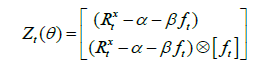
Where, is the 10 x 1 vector containing the excess returns of the stocks sorted in tendecile portfolios, is the 10 x 1 vector containing the intercept of the model, is and is an additional risk factor used to capture the size effect. The errors εt in vector form are presented as

The equation (2.3) can be rewritten as below:

(2.4)

Where,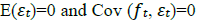

If the set of unknown parameters (α, β) is denoted by θ. Then the GMM estimator of θ minimizes the following quadratic equation form:

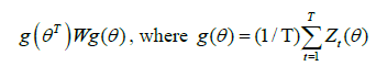(2.5)

Where, the estimator of the weighting matrix (W) is used to identify the problem of autocorrelation and heteroscedasticity. For the estimation of W, the method of Newey and West’s (1987) is employed (Newey and West, 1987 ). Thus, the GMM moment’s conditions can be defined as:

(2.6)

This equation is used to interpret the results which cause the return model to accept or reject. For example, the efficiency of "f_t" imply that alpha (α) is approximately equals to zero. This zero value of alpha leads us to make interpretation regarding the profitability of the size effect with reference to CAPM. That is, in the case of zero value of alpha (α), it insures the validity of CAPM. In other words, there is no evidence of predictable pattern for example, small size effect on the stock market. While any positive value of alpha leads us to develop a view that size effect exists to determine the stock returns (Kashif, 2013) .

Appendix 3

Construction of Mimicking Portfolios for SMB, HML, RMW and CMA Factors

To construct the portfolios for the Fama-French three-factor model, we followed mimicking portfolio construction used by Fama and French (1993) . The size factor data was divided into two sub-groups, small (S) and big (B) market capitalization firms, by using median as a breakup point and book-to-market equity factor data was divided into three sub-groups, high (H), neutral (N) and low (L) book-to-market equity firms, by using 30th and 70th percentiles as breakup points. The portfolios were made on 2x3 sort; where SMB factor is a simple average of returns on small market capitalization portfolios, minus big market capitalization portfolios and the HML factor is a simple average of returns on high book-to-market equity portfolios minus low book-to-market equity portfolios. On the basis of 2x3 sort of SMB and HML factors the six portfolios formed, are as under:

SH=Portfolio of small market capitalization firms and high book-to-market equity ratio firms.

SN=Portfolio of small market capitalization firms and neutral book-to-market equity ratio firms.

SL=Portfolio of small market capitalization firms and low book-to-market equity ratio firms.

BH=Portfolio of big market capitalization firms and high book-to-market equity ratio firms.

BN=Portfolio of big market capitalization firms and neutral book-to-market equity ratio firms.

BL=Portfolio of big market capitalization firms and low book-to-market equity ratio firms.

The construction of portfolios for the Fama-French five-factor model, the study used 2x3 sort, used by Fama and French (2015). The size factor and book-to-market factor data were divided into 2 and 3 categories similarly to three-factor model. The profitability factor data was divided into three sub-groups, robust (R), neutral (N) and weak (W) operating profitability firms, by using 30th and 70th percentiles as breakup points. Moreover, the investment factor data was also divided into three sub-groups, conservative (C), neutral (N) and aggressive (A), same like the previous factors by using 30th and 70th percentiles as breakup points. Here, the construction of size factor is different from the three-factor asset pricing model. The size factor (SMB) was constructed by subtracting nine portfolios of big stocks from nine portfolios of small stock. On the basis of 2x3 sort, the study formed eighteen portfolios, are as under:

SH=Portfolio of small market capitalization firms and high book-to-market equity ratio firms.

SN=Portfolio of small market capitalization firms and neutral book-to-market equity ratio firms.

SL=Portfolio of small market capitalization firms and low book-to-market equity ratio firms.

BH=Portfolio of big market capitalization firms and high book-to-market equity ratio firms.

BN=Portfolio of big market capitalization firms and neutral book-to-market equity ratio firms.

BL=Portfolio of big market capitalization firms and low book-to-market equity ratio firms.

SR=Portfolio of small market capitalization firms and robust profitability firms.

SN=Portfolio of small market capitalization firms and neutral profitability firms.

SW=Portfolio of small market capitalization firms and weak profitability firms.

BR=Portfolio of big market capitalization firms and robust profitability firms.

BN=Portfolio of big market capitalization firms and neutral profitability firms.

BW=Portfolio of big market capitalization firms and weak profitability firms.

SC=Portfolio of small market capitalization firms and conservative investment firms.

SN=Portfolio of small market capitalization firms and neutral investment firms.

SA=Portfolio of small market capitalization firms and aggressive investment firms.

BC=Portfolio of big market capitalization firms and conservative investment firms.

BN=Portfolio of big market capitalization firms and neutral investment firms.

BA=Portfolio of big market capitalization firms and aggressive investment firms

Construction of Size, Book to Market Value, Profitability and Investment factors is explained as follows.

Size Factor (SMB)

For three-factor asset pricing model, the study follows Fama-French (1993) mimicking portfolio construction and for the five-factor model, we use 2x3 sort of portfolios constructed by Fama and French (2015). The construction of SMB factor for three-factor asset pricing model is given in equation as follow:

And, the construction of SMB factor for five-factor asset pricing model is given in equation as follows:

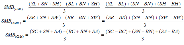
For five-factor asset pricing model, first the study has to construct three size factors by taking weighted averages on the basis of book-to-market, profitability and investment factors than construct the final size factor for the model by taking an average of all sub-factors, see Fama and French (2015).

Book to Market Value Factor (HML)

For both three-factor and five-factor model the construction of HML factor is the same which is as follows:

Profitability Factor (RMW)

For the construction of portfolios for profitability, the study used 2x3 sort also used by Fama and French (2015) . The construction formula is given as follow:

Investment Factor (CMA)

The construction of the investment factor is given as follow:

Endnotes

1. The intrinsic valve is the present value of the cash flows; the owner of the stock expects to receive (Bodie et al., 2009).

2. Risk adjusted return is a measure of return on an investment at given level of risk associated with it. Usually, it is used to compare the returns of portfolios with similar risk characteristics (Bodie et al., 2009) .

3. Banz (1981) believes that the size effect is stable throughout the time period by using the stock listed in NYSE.

4. Stehle (1997) shows modest size effect in 1950’s and strong size effect in the 1970’s and late 1980’s in German Stock market. Korolenko and Betan (2006) used Stehle’s report just to give more insight to crises period for the existence of size effect.

5. Survivorship biases rise in the average returns of a sample of companies when some failed companies are excluded on the basis of their poor performances from the sample period (Bodie, 2009).

6. Mnemonic is special individual code for each data series. (Thomson Reuters DataStream).

7. Market Value (MV) is defined as the total number of shares multiplied by its price. It is also mandatory for the calculation of value weighted returns (Thomson Reuters DataStream).

8. Rebalancing means to update the sorting criteria informative every month.

References

1. Ali, R., & Khan, R.E.A. (2018). Socioeconomic stability and variability in stock market prices: A case study of Karachi stock exchange. Asian Journal of Economic Modelling, 6(4), 428-440.
2. Anigbogu, U.E., & Nduka, E.K. (2014). Stock market performance and economic growth: Evidence from Nigeria employing vector error correction model framework. The Economics and Finance Letters, 1(9), 90-103.
3. Balakrishnan, A. (2016). Size, value, and momentum effects in stock returns: Evidence from India. Vision: The Journal of Business Perspective, 20(1), 1-8.
4. Banz, R.W. (1981). The relationship between return and market value of common stock. Journal of Financial Economics, 9, 3-18.
5. Basu, S. (1981). The relationship between earning yields, market value and return for NYSE Common Stocks: Further evidence. Journal of Financial Economics, 12 (1), 129-156.
6. Berk, J.B. (1995). A critique of size-related anomalies. The Review of Financial Studies, 8, 275-286.
7. Black, F., Jensen, M., & Scholes, M. (1972). The capital asset pricing model: Some empirical tests, in Michael C. Jensen (eds), Studies in the Theory of Capital Market. New York: Praeger.
8. Bodie, Z., Kane, A., & Marcus, A.J. (2009). Investments, (Eighth Edition).McGraw-Hill, US.
9. Brown, P., Kleidon, A.W., & Marsh, T.A. (1983). New evidence on the nature of size related anomalies in stock prices. Journal of Financial Economics, 12, 33-56.
10. Campbell, J.Y., Lo, A.W., & Mackinlay, A.C. (1997). The econometrics of financial markets. Princeton, USA.
11. Chaibi. A., Alioui. S., & Xiao. B (2014). On the impact of firm size on risk and return: Fresh evidence from the american stock market over the recent years. Journal of Applied Business Research, 31, 29-36.
12. Clare, A., & Thomas, S. (1995). The overreaction hypothesis and uk stock market. Journal of Business Finance and Accounting, 22, 961-73.
13. Cochrane, J.H. (2005). Asset pricing. Princeton University Press.
14. Conrad, J., & Kaul, G. (1988). Time variation in expected returns. Journal of Business, 61, 409-25.
15. Corhay, A., Hawawini, G., & Michael, P. (1988). The pricing of equity on the London exchange, seasonality and size premium, stock market Anomalies. InE. Dimson (ed), Cambridge University Press.
16. Dasgupta, R. (2014). Driving role of institutional investors in the indian stock market in short and long-run an empirical study. International Journal of Business, Economics and Management, 1(6), 72-87.
17. Dijk, M.V. (2011). Is size dead? A review of the size effect in equity returns. The Journal of Banking and Finance, 35, 3263-3274.
18. Dimson, E., & Marsh, P. (1999). Murphy’s law and market anomalies. The Journal of Portfolio Management, 25, 53-69.
19. Elfakhani, S., Lockwood, L.J., & Zaher, T.S. (1998). Small firm and value effects in the canadian stock market. Journal of Financial Research, 21, 277-91.
20. Fama, E.F. (1991). Efficient market hypothesis. The Journal of Finance, 46, 383-417.
21. Fama, E.F., & French, K.R. (1992). The cross-section of expected returns. The Journal of Finance, 33, 3-56.
22. Fama, E.F., & French, K.R. (1993). Common risk factors in the returns on stocks and bonds. Journal of Financial Economics, 33, 3-56.
23. Fama, E.F., & French, K.R., (1996). Multifactor explanations of asset pricing anomalies. Journal of Finance, 51, 55-84.
24. Fama, E.F., & French K.R. (2004). The capital asset pricing model. Journal of Economic Perspectives, 18, 25-46.
25. Fama, E.F., & French, K.R. (2008). Dissecting anomalies. Journal of Finance, 63, 1653-1678.
26. Fama, E.F., & French, K.R. (2012). Size, value, and momentum in international stock returns. Journal of Financial Economics, 105, 457-472.
27. Fama E.F., & French, K.R. (2015). A five-factor asset pricing model. Journal of Financial Economics, 116, 1- 22.
28. Fletcher, J., & Kihanda, J. (2005). An examination of alternative CAPM-based models in UK stock returns. Journal of Banking and Finance, 29, 2995-3014.
29. Florackis, C., Gregoriou, A., & Kostakis, A. (2011). Trading frequency and asset pricing on the london stock exchange: Evidence from a new price impact ratio. Journal of Banking and Finance, 35, 3335-50.
30. Fraser, P. (1995). Returns and firm size: A note on the uk experience 1970-1991. Applied Economics Letters, 2, 331-334.
31. Furqan, M., & Sharif, S. (2015). Impact of size on return at karachi stock exchange (KSE). Retrieved from https://papers.ssrn.com/sol3/papers.cfm?abstract_id=2605460
32. Gibson, G. (1889). The stock markets of London. Paris and New York.
33. Gregory, A., Harris, R.D., & Michou, M. (2001). An analysis of contrarian investment strategies in the UK. Journal of Business Finance & Accounting, 28(9?10), 1192-1228.
34. Grossman, S.J., & Stiglitz, J.E. (1980). On the impossibility of informationally efficient markets. The American Economic Review, 70, 393-408.
35. Haq, I., & Rashid, K. (2014). Stock market efficiency and size of the firm: Empirical evidence from Pakistan. Economics of Knowledge, 6, 10-31.
36. Herrera, M.J., & Lockwood, L. (1994). The size effect in the mexican stock market. Journal of Banking & Finance, 18, 621-632.
37. Heston, S.L., Rouwenhorst, K.G., & Wessels, R.E. (1999). The role of beta and size in the cross-section of european stock returns. European Financial Management, 5(1), 9-27.
38. Horowitz, J.L., Loughran, T., & Savin, N.E. (2000). The disappearing size effect. Research in Economics, 54, 83-100.
39. Hsieh, T.Y., Lee, H.I., & Tsai, Y.R. (2018). Idiosyncratic risk, stock returns and investor sentiment. Asian Economic and Financial Review, 8(7), 914-924.
40. Hussain, S. (1996). Over?reaction by security market analysts: The impact of broker status and firm size. Journal of Business Finance & Accounting, 23(9?10), 1223-1244.
41. Inusah, N. (2018). Toda-yamamoto granger no-causality analysis of stock market growth and economic growth in ghana. Journal of Accounting, Business and Finance Research, 3(1), 36-46.
42. Jamali, A.H., Asadi, A., & Asnavandi, M. (2012). The study of improvement of the level of access to capital market on efficiency of tehran stock exchange. International Journal of Asian Social Science, 2(8), 1193-1202.
43. Jegadeesh, N. (1990). Evidence of predictable behavior of security returns. The Journal of Finance, 45, 881-898.
44. Jensen, M. (1968). The performance of mutual funds in the period 1945-64. The Journal of Finance, 23, 389- 416.
45. Kashif, M. (2013). The pricing of coskewness and cokurtosis risks on the UK stock market. Ph.D. Thesis, University of Glasgow.
46. Kato, K., & Schallheim, J.S. (1985). Seasonal and size anomalies in the japanese stock market. Journal of Financial and Quantitative Analysis, 20, 243-260.
47. Keim, D.B. (1983). Size-related Anomalies and Stock Return Seasonality. Journal of Financial Economics, 12, 13-32.
48. Kendall, M. (1953). The analysis of economic time series. Journal of the Royal Statistical Society, 96, 11-25.
49. Khan, N., Ali, K., Kiran, A., Mubeen, R., Khan, Z., & Ali, N. (2016). Factors that affect the derivatives usage of non-financial listed firms of pakistan to hedge foreign exchange exposure. Journal of Banking and Financial Dynamics, 1(1), 9-20.
50. Klein, R.W., & Bawa, V.S. (1977). The effect of limited information and estimation risk on optimal portfolio diversification. Journal of Financial Economics, 5, 89-111.
51. Korolenko, M., & Betan, J. (2006). War, crisis, and the capital market: The anomaly of the size effect in germany, 1872-1990. International Economic History Congress, Session 20.
52. Kostakis, A., Kashif, M., & Siganos, A. (2012). Higher co-moments and asset pricing on london stock exchange. Journal of Banking and Finance, 36, 913-922.
53. Lakonishok, J., & Shapiro, A.C. (1986). Systematic risk, total risk, and size as determinants of stock market returns. Journal of Banking and Finance, 10, 115-132.
54. Lakonishok, J., Shleifer, A., & Vishney, R.W. (1995). Contrarian investment, extrapolation, and risk. Journal of Finance, 50, 541-78.
55. Le, H.L., Vu, K.T., Du, N.K., & Tran, M.D. (2018). Impact of working capital management on financial performance: The case of Vietnam. International Journal of Applied Economics, Finance and Accounting, 3(1), 15-20.
56. Lee, C.H., & Chou, P.I. (2018). Corporate cash holdings and product market competition: The effects of stock-based executive compensation. Asian Economic and Financial Review, 8(9), 1140-1157.
57. Levis, M. (1985). Are small firms big performers? The Investment Analysis, 76, 21-27.
58. Lin, J.B., Onochie, J.I., & Wolf, A.S. (1999). Weekday variations in short-term contrarian profits in futures markets. Review of Financial Economics, 8(2), 139-148.
59. Lintner, J. (1965), The valuation of risk assets and the selection of risky investments in stock portfolios and capital budgets. The Review of Economics and Statistics, 47, 13-37.
60. Lo, A.W., & Mackinlay, A.C. (1988). Stock market prices do not follow random walks: Evidence from a Simple Specification Test. Review of Financial Studies, 1, 41-66.
61. Malkiel, B.G. (2003). The efficient market hypothesis and its critics. Journal of Economics Perspective, 17, 58-82.
62. Markowitz, H. (1952). Portfolio selection. Journal of Finance, 7(1), 77-91.
63. Mirza, N., & Shahid, S. (2008). Size and value premium in karachi stock exchange (KSE). The Lahore Journal of Economics, 13, 1-26.
64. Newey, W.K., & West, K.D. (1987). A simple, positive-definite, heteroskedasticity and autocorrelation consistent covariance matrix. Econometrica, 55, 703-708.
65. Nzimande, N., & Padayachee, P. (2017). Evaluation of the current procurement planning process in a district municipality. International Journal of Public Policy and Administration Research, 4(1), 19-34.
66. Oluwaseun, G.O., & Boboye, L.A. (2017). Randomness of stock return in nigerian banking sector. Asian Journal of Economics and Empirical Research, 4(2), 99-105.
67. Rauf, A.L.A. (2016). Risk and return: Comparative study of active sukuk markets of Nasdaq HSBC amanah sukuk and nasdaq Dubai listed sukuk. Global Journal of Social Sciences Studies, 2(2), 104-111.
68. Reinganum, M. (1981). Misspecification of capital asset pricing: Empirical anomalies based on earnings yields and market value. Journal of Financial Economics, 9, 19-46.
69. Riro, G.K., & Wambugu, J.M. (2015). A test of asset-pricing models at the nairobi securities exchange. Research Journal of Finance Accounting, 6(2).
70. Robert, H. (1959). Stock market patterns and financial analysis. Journal of Finance, 14, 1-10.
71. Sabri, T.B.H., & Sweis, K.M. (2015). The impact of the global financial crisis on the debt, liquidity, growth, and volume of companies in palestine stock exchange. Journal of Social Economics Research, 2(2), 31-37.
72. Salim, M.N., & Hariandja, N.M. (2018). Factors affecting joint stock price index (CSPI) and the impact of foreign capital investment (PMA) Period 2009 to 2016. Humanities and Social Sciences Letters, 6(3), 93-105.
73. Schwert, G.W. (2002). Anomalies and market efficiency. Working Paper, University of Rochester.
74. Sharpe, W.F. (1964), Capital asset prices: A theory of market equilibrium under conditions of risk. Journal of Finance, 19, 425-442.
75. Sharpe, W.F., Gordon, J.A., & Baley, J.V. (1999). Investments, (Sixth Edition).Upper Saddle River.
76. Soares, N., & Stark, A.W. (2009). The accruals anomaly can implementable portfolio strategies be developed that are profitable net of transactions costs in the UK? Accounting and Business Research, 39, 321-45.
77. Stehle, R. (1997). The size affect on the German stock market. Zeitschrift fur Bankrecht und Bankwirtschaft, 9, 237-260.
78. Strugnell, D., Gilbert, E., & Kruger, R. (2011). Beta, size and value effects on the JSE, 1994-2007. Investment Analysts Journal, 40, 1-17
79. Tahir, S.H., Sabir, H.M., Alam, T., & Ammara, I. (2013). Impact of firms characteristics on stock returns: A case of non- financial listed companies in pakistan. Asia Economics and Financial Review, 3, 51-61.
80. Ullah, F., Hussain, I., & Rauf, A. (2014). Impacts of macroeconomy on stock market: Evidence from Pakistan. International Journal of Management and Sustainability, 3(3), 140-146.
81. Waheed, A., Yang, J., Ahmed, Z., Rafique, K., & Ashfaq, M. (2017). Is marketing limited to promotional activities? The concept of marketing: A concise review of the literatur. Asian Development Policy Review, 5(1), 56-69.
82. Wong, K.A., & Lye, M.S. (1999). Market value, earning yields and stock returns: Evidence from Singapore. Journal of Banking and Finance, 14, 311-326.