Research Article: 2021 Vol: 24 Issue: 6S
Automatic Lip Reading Classification Using Artificial Neural Network
Ahmed K. Jheel, University of Babylon
Kadhim M. Hashim, University of Babylon
Abstract
Lip Reading depends on watching the shape of speaker's mouth region ; Especially his lips to understand the letters and words that have been uttered through the movement of the lips, gestures and expressions on the face, the location of the lips and its extracted features. This paper presents a new system include some of stages applied to AV Letters 2 dataset. The first three stages are preprocessing,face\lip detection,lip localization based on a set of new approaches that aims to get region of interest (or lip region) accurately and clearly with the help of new techniques and other operation of image processing. This paper focus on the last two stages of the automatic lip reading system: features extraction and classification. There are three various sets of distinguished features as (SURF, Centroid, HOG) are used in the proposed system. These features give a set of points called key points are exactly located on the lip borders that have been tracked using Euclidean distance calculation. The classification performs using artificial neural network to be a new one of the visual speech recognition tools.
Keywords
Lip Reading, Face Detection, Feature Extraction, SURF, Classification, Neural Network
Introduction
This paper proposes a system for automatic lips reading for the English language. Simple linguistics units are chosen (vowels) and a robust system for feature extraction is created and analyzed. The entire system is built from two basic operations. The first operation introduces feature extraction from video sequences of spoken vowels letters and the second one represents classification phase. Feature extraction is performed in several steps: face detection, lip detection, lip localization, feature extraction. The aim is to construct a design which consists of several stages, that follow sequentially and they supplement each other. The stage of lips detection seems to be most important part of proposed design. The pre-processing stage that starting with frames sequence of video where each frame needs many methods should be used to maintain information about their position through the whole sequence deployed for this purpose. The last stage of our design proposes classification using artificial neural network based on feature extraction which provides scale -space robustness. The all process is steadied on and which serves as good proof for recognition of proposed lips reading design.
The Proposed System
In recent a significant amount of research has been directed towards automatic lip reading field. Since one of the most important applications of LR is surveillance for security purposes, which involves real-time recognition of lip from a frame sequence captured by a video camera. Automatic lip-reading technology plays a vital role in human language communication and visual perception. An integral lip-reading system is an automatic method developed to locate the lips from the face of the speaker without sounds for extracting visual information from the sequence of frame of input video to track it in consecutive frames to speech recognition.
In this section, the proposed framework of lip reading is implemented by several stages to be done as shown in Figure (1). It will be discussed in detail. There are following six stages are applied on the front view of the four speakers in the AV letters 2 Dataset to identify what they said.

Figure 1: The General Diagram of the Proposed System
The figure shown above, the most important stages that makes up the system for the purpose of obtaining the spoken letter. Each of these stages includes a set of processes and multiple ways to implement them; each stage depends on the results of the preceding stage.
At the first stage, before going into the proposed system, a pre-processing must be carried out at the beginning where the original video is divided into a number of frames, creating an RGB mask for each frame and then converting it into an HSV color space.
At the second stage, it requires obtaining the face area for the purpose of obtaining the lip area that is the most important area for the purpose of reaching the goal of the system. Each frame is transformed from HSV color space to binary mask, and then determining the centroid of the white area, the major axis length and the minor axis length, from it an ellipse is created, where the center of an ellipse equal to the centroid, and thus the face area is obtained after multiplying it with the original image.
At the third stage will be extract ROI by segmenting the ellipse face in to there after that extract features in the fourth stage that represented by set of key points that tracing in instructive frames produced in the fifth stage. The final stage will be the classification. It will be explained in detail in this chapter. The figure (1) shows the block diagram of the proposed system. The first three stages had been discussed in details in our Research (Khleef et al, 2021). This paper interested with the last two stages: feature extraction and classification as completely for the previous research.
Feature Extraction
Feature extraction is the fourth stage in the system and allows us to highlight information of interest from the images to represent a target. In this section, will introduce the image formation process and discuss the employed methods to extract features that are significant for the disambiguation of the objects of interest and to study how these features are combined. Features (descriptors or signatures) describe an important image characteristic that are produced in the video sequence and before being transferred to classification stage. We combine three features: SURF, HOG, centroid, height and width of lips feature is a new idea used to feature extraction. Now we discussed in details the categories of these features as shown in figure (2).

Figure 2: The Selective Types of Features Extraction
Centroid
In physics and mathematics, the centroid or geometric shape of a shape is the average location of all points in the geometric shape. Unofficially, it is the point at which the shape outage can be perfectly balanced on the tip of a pin (Protter, 1970).
The definition extends to any object in n-dimensions space: its centroid is the average position of whole points in all directions of coordinates (Priyanka, 2014).
While in geometry, the term barycenter is equivalent with centroid, in astrophysics and astronomy, barycenter is the center of the mass of two or more bodies orbiting each other see figure (3). The standard formula for the centroid of a two dimensional object (or image) is given by;

Figure 3: (A) Show the Singular Centroid When the Mouth is Closed (B),(C) Show Two Centroids When the Mouth is Opened
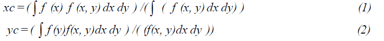
Where (xc, yc) are the centroid coordinates and If(x, y) is the function defining the two dimensional object. In discrete form the equations can be written as;
This equation is applied to the all frames and gives good results successfully. As result, the central point of a limited set of points is this point reduces the sum of the square Euclidean distances between them and each point in the set.
As result, we note by applying the centroid to the mouth region, there is at most two points will be obtained in the case of the opened mouth as a result of the formation of two areas represented by the outer real contour of the mouth and the area of the internal contour of the mouth see figure (3/b,c).
Histogram of Gradient (HOG)
The same representation used to encode the color information in the target area can be applied to other low-level features, such as the image gradient. The image gradient highlights strong edges in the image that are usually associated with the borders of a target. To use the image gradient in the target representation, one can compute the projection of the gradient perpendicular to the target border or the edge density near the border using ambinary Laplacian map. However, these forms of representation discard edge information inside a target that may help recover the target position, especially when the target appearance is highly characterised by a few texture patterns. More detailed edge information can be obtained from the histogram of the gradient orientation, also known as orientation histograms Implementation of the HOG descriptor algorithm is as follows:
1. Divide the image I into small connected regions called cells, and for each cell compute a histogram of gradient directions or edge orientations for the pixels within the cell. Gradient. Approximate the two components Ix and Iy of the gradient of I by central differences1:

While convolution with a Gaussian derivative produces higher efficiency derivatives in the presence of noise, the smoothing that this convolution implies removes valuable details. Furthermore, some noise will occur in later stages of the HOG calculation when histograms are calculated so that Gaussian smoothing is both less helpful and unusually costly. The gradient is converted into a polar co-ordinate with an angle between 0̊ and 180̊, to identify gradients pointing in opposing directions.

Where tan−1 is the four-quadrant inverse tangent, which yields values between −π and π.
2. Discretize each cell into angular bins according to the gradient orientation. Each cell's
pixel contributes weighted gradient to its corresponding angular bin. This referred to
cell orientation histograms. Partitioning the window into adjacent, non-overlapping
cells of size C × C pixels (C=8). Calculate a histogram of the gradient orientation in
each cell and then binned into bins B (B=9). With so few bins, an image with a pixel
whose orientation is close to a bin boundary might end up contributing to a different
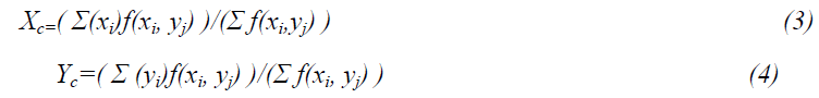
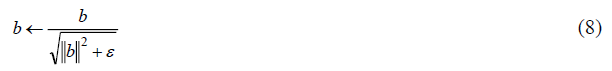
bin. Was the image to change slightly? To avoid these quantization devices, each pixel in a cell contributes to two adjacent bins (modulo B) a fraction of the pixel’s gradient magnitude µ that decreases linearly with the distance of that pixel’s gradient orientation from them won in centers (Figure 4). Specifically, the bins are numbered 0 through B-1 and have width Bin has boundaries and centers a pixel with magnitude µ and orientation θ contributes a vote
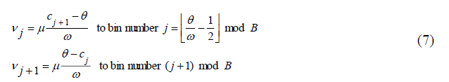

Figure 4: This Scheme is Called (for Dubious Reasons) Voting by Bilinear Interpolation and is Illustrated In Figure 2. The Resulting Cell Histogram is a Vector with b Nonnegative Entries
3. Block Normalization: Group the cells into overlapping blocks of 2 × 2 cells each, so that each block has size 2C × 2C pixels. Two horizontally or vertically consecutive blocks overlap by two cells, that is, the block stride is C pixels. As a consequence, each internal cell is covered by four blocks. Concatenate the four cell histograms in each block into a single block feature b and normalize the block feature by its Euclidean norm as described in equation (8):
In this expression, is a small positive constant that prevents division by zero in gradient-less blocks? The evidence for preferring this normalization scheme over others is entirely empirical.
4. Groups of adjacent cells are considered as spatial regions grouping and normalization of histograms. In other words normalization of Block is a compromise, Cell histograms, should be normalized to minimize the effects of variation in contrast between images of the same object. On the other hand, the overall gradient magnitude carries certain information and normalization across a block, a region larger than one cell preserves piece of this information, specifically the relative gradient magnitudes in the cells of the same block. Since each cell is covered by up to four blocks, each histogram is represented up to four times with up to four different normalizations.
5. Normalized group of histograms represents the block histogram. The set of these block histograms represents the descriptor. HOG Feature. Normalized block features are concatenated into a single HOG feature vector h, which is normalized as follows:
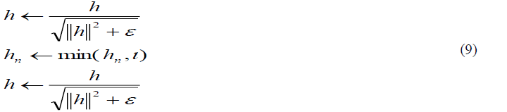
Here, hn is the n-th entry of h and τ is a positive threshold (τ=0.2). Clipping the entries of h to be no greater than τ (after the first normalization) ensures that very large gradients do not have too much influence they would end up washing out all other image detail. The final normalization makes the HOG feature independent of overall image contrast. The following figure demonstrates the algorithm implementation scheme:

Figure 5: Represent the Steps of Hog Implemention
| Algorithm (1) Computation of HOG |
|---|
| Input: image I(x, y), block size(C). |
| Output: HOG feature. |
| Step1: Divide I(x, y) into small adjacent non - overlapping block (2C × 2C), each block has (2 × 2)cells. For i=1 to No. of block do. For j=1 to No. of cell do |
| Step 2: Compute the gradient in two directions Ix, Iy by central differences (use equation (5)). |
| Step 3: Compute the magnitude of gradient and its orientation |
| Step 4: Discretize each cell into angular bins (B=9) according to the gradient orientation. Since each cell's pixel contributes weighted gradient to its corresponding angular bin. |
| Step 5: Compute a histogram of the gradient (HOGj ) its orientation for each cell and binned into bins. |
| Step 6: Use voting by bilinear interpolation (vi) when a pixel whose orientation is close to a1bin boundary might end up contributing to a differentibin (see equation (7)) |
| Step 7: Group each resulted HOGj from the previous step into block (bi). And normalize the (bi) by its Euclidean norm (use equation (8)). |
| Step 8: Concatenate the normalizednblocknfeatures (bi) into a single HOGi feature vector h, and then normalized. |
| [ Add to final HOG vector] |
| End for |
| End for |
| End algorithm |
Algorithm 1 Represent Computation of Hog Algorithm
In general, it is desirable to have a representation that is invariant to target rotations and scale variations:
Invariance to rotation is achieved by shifting the coefficients of the histogram according to θ, the target rotation associated with a candidate state x.
Scale invariance is achieved by generating a derivative scale space. The orientation histogram of an ellipse with major axis h is then computed using the scale-space- la d l v l σ closest to h/R, where R is a constant that determines the level of detail, where R is a constant that determines the level of detail, as result we obtain.
Speed UP Robust Feature (SURF)
The SURF algorithm may be split into six stages as shown in (Figure 6). This section attempt to explain its basic calculation in details to understand these interest point descriptor and its uses in digital image processing field.

Figure 6: Illustrate the Stages of the Surf Algorithm
The SURF feature is based on a approximation of Hessian matrix (Ke, 2004). This allows for the usage of integral image, which minimize the computational time significantly. In the instance of SURF interest point’s detector, the Hessian matrix was estimated approximately in constant time using 9 × 9 simple box filters. The integral images form of representation used by SURF enables for quick calculation of box convolution filters. The sum of entire pixels in the original picture I inside a rectangle area defined by the origin and X represent the integral image IΣ(X) placed at X=(x, y)T.
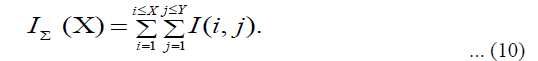
Where X is the width of an image and Y is the height of an image.
The most distinctive feature of integral image is that it tends to reduce processing time of pixel values resulting faster computations in square regions (as shown in Figure 7). To compute the total I∑abcd independently on filter scale, three arithmetical operations are required as shown in Equation (10).


Figure 7: Integral Image Illustration
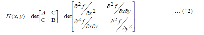
The Hessian matrix is generated at the second stage of the SURF algorithm by using 2nd order Gaussian filter in x and y directions. The pixel values that correspond to the black rectangles are taken from the white rectangle values. The black rectangle pixel values have been doubled, and then subtracted from the white rectangle pixel values. The following equation is used to calculate the Hessian determinant.
The real Gaussian kernels do not have a discrete form but it has a continuous function [10]. Instead, a Gaussian kernel approximation is employed. The equation for computing the determinant of Hessian using an approximated Gaussian kernel is:

For balancing the Hessian's determinant need to employ the filter responses were weighted using the relative weight w. This is required to preserve the available Gaussian kernel energy.
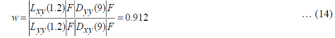
Where |x|F is the Frobenius norm,1w24 is a weight Coefficient equal to 0.83. In hardware it is good idea to use. w2=1–1/8.=0.875, because the subtraction 1/8 portion is simple to implement.
The determinant responses to scale are normalized in the third. Stage of this algorithm the greater scale allows more pixels enter the kernel. And more determinant responses are obtained. When non-maximal suppression was applied, this reduces the probability of discovering distinct features at a higher scale (Birchfield, 1998).
The non-maximal suppression is computed in the fourth stage. It's based on determining the greatest determinant value. Among 26 closest neighbors in the lower, current, and higher scales. Following that, the value is filtered using a preset threshold to hold just the strongest points.
The Haar wavelet in x and y directions of size 4σ are computed for the assignment of orientation at the fifth stage. Wavelets are calculated for pixels that lied within a radius of 6σ around the point of interest (Figure 8).
The prominent orientation is assessed by the sum of vertical and horizontal responses.
At the last stage, the descriptor is computed utilizing Haar wavelets in square 20σ size area centered at the point of interest and oriented along the prominent direction.

Figure 8: Illustration of the Scaled and Orientated Grid r. the Grid r, Divided Into 16 Subregions, is Used to Build the Surf Descriptor in the Neighborhood of an Interest Point xk: (xk, yk, lk) with Orientation k
Tracing Lips in the Consecutive Frames
As it's known, the proposed automatic lip reading is visual signal at time in the video sequences, and the whole task is executed on series of consecutive frames. Therefore it is necessary to design effective algorithms, because of large amount of data. Suppose the information about lips position in each image (video frame) can enhance the effectiveness of lips reading. Generally two basic approaches can be used for this purpose:
• Searching for lips in each frame.
• Tracking lips over all frames.
Searching for lips is not trivial, this process is time consuming and not always efficient (lip localization stage showed many difficulties of this process). Therefore lips tracking algorithm in our model as follow:
Through the feature extraction stage, 160 coordinate points have been obtained from three features (centroid, SURF, HOG)). Now, the detected points from the first frame to the last one must be tracked in the following frames block by block. In this method the Euclidean distance between each frame is calculated with the preceding frame. As already know that each input video represent a single utterance of letter and divided into its frame. If input video consist of 30 frames for example, and from each frame has 160 detected points were obtained, then as a final result, each utterance is represented by a matrix of 160 x 30 in which each column detect the single point movement in the following frames see figure (9). It uses two steps. They are as follows.

Figure 9: (A) Show the Singular Centroid when the Mouth is Closed
a. In various directions POI will be tracked to detect the POI movements in the following frames, and Euclidian distance are derived.
b. Calculate the coefficient of variances for the Euclidian distance Among frames for individual each point.
Here, to trace the lips in the following frames of the video the same procedure is not repeated as such in the first frame. Using the key points that have been obtained in the previous step, easily tracking is done in the next frames by finding their positions with the Euclidean distance.
The Classification
From all the previous features, the features (centroid, SURF, HOG) are selected for classifying by using the artificial neural network which represented by162 coordinate points. In general, each of selected features have different numbers of points such as (centroid=2 points, SURF=60 points, HO=100 points). And these features actually represent the strongest points for each frame for utterance of the single letter. From each frame there are 162 cumulative features (from the first frame to the last frame of single letter). Suppose that every utterance contains 162 features and its frames number (N) that varies in size according to the different speed pronunciation and the letter it. Thus, each letter will be represent as a matrix which dimension is N×162, where N represents the number of frames for the single letter.
The feature matrix has a fixed number of columns (162 in all cases), but with a different number of rows (depending on number of frames). Therefore; the following procedure is used:
1. The Euclidean distance between the frames' key points was calculated, which meaning the Euclidean distance between the frame (n) and the frame (n+1) is calculated to represent the changes for each point in the first frame to the last frame
2. After completing the calculation of the Euclidean distance for all the key points in the feature matrix which represented by columns.
3. The Euclidean distance between frames' key points will be tracked
4. Take the coefficient of variances of these distances to reduce the dimensionality, thus, the feature matrix will be converted into a vector (meaning that each value in the vector represents the average of the Euclidean distances of first point from the first frame to the last frame and the second value in the vector represents the average of the Euclidean distances of the second point, from the first to the last frame, and so on) applying for all the points that represent the letter.
Now there are four speakers in AVletters2 Dataset. Every one of them uttered the 26 English vowel letters seven times. So the number of pronounced letters is 5 × 7 × 4=140. 4 represent the number of speakers, 7 represent the number of times a single letter is spoken, and 5 represent the number of vowels in the English language. As mentioned earlier, each spoken letter will be represented by one vector of length 162. There are 140 vectors divided into five equal sets. Each group consisting of 28 vectors that represent each vowel letters. For the fusion of the aforementioned features, researchers reported three types of fusion: Feature-based fusion, score level fusion and decision-based fusion (Potamianos et al., 2003). Simple features concatenation is an example of feature-based fusion methods, where all the features vectors concatenated in one feature vector, which is passed as it is to the recognizer, or is transformed using appropriate transformation then passed to the recognizer. Applying such fusion in our approach is problematic for several reasons; first, the signal length will be 8 times longer than the normal length, so comparing signals becomes time inefficient, Second, all the features will contribute equally to the final results, and while they are not equally representative, some features are not as representative as others.
The features vector normalized to the range (Schaeferling, 2011) to alleviate the individual differences, and different scales of mouth caused by different distances from the camera, i.e., the different sizes of ROIs. For each property, a feature vector (a signal) is obtained to represent the spoken word from that feature perspective
In this chapter using artificial neural network as classifier to map phonemes to corresponding visemes. It is not necessary to have a unique viseme for every phoneme, since there are several phonemes that have the same or similar facial expression (Liu & Chen, 2004). A multilayer back-propagation artificial neural network as shown in Figure (10) is used with sigmoid activation function. Artificial Neural network classifies input phonemes to generate corresponding viseme. Artificial neural network have been created to test and train phonemes. Each ANN was created with different combinations of 162 input neurons, two hidden layer of 50 neurons and the output layer with three neurons. The number of output neuron based on letters spoken. Every letters should be represented in binary digits. we have five letters ('A', 'E', 'I', 'O', 'U' ) will be represented by three binary digits (001, 010, 011, 100, 101) and then coded to ASCII code (65, 69,73, 79, 85).

Figure 10: Artificial Neural Network
Results
In this section, we demonstrate our proposed method using AVLetters2 database (Freeman and M. Roth, 1995) to estimate the performance for mouth localization and speech recognition from frontal video. The face frame has 1920 × 1080 in size and frontal pose in addition to each video contain 50 fps. All experiments worked in a 2.80 GHz Intel ® Core(TM) is-2300 CPU with 4 GB RAM PC and MATLAB programs. And the computational time of mouth detection is about 0.60s with size of 320× 250 for a face frame. Now there are four speakers in AVletters2 Dataset. Every one of them uttered the 26 English vowel letters seven times. So the number of pronounced letters is 5×7×4=140, (4) represents the number of speakers, (7) represents the number of times a single letter is spoken, (5) represents the number of vowels in the English language and the result was as follow Table 1.
| Table 1 Error Reduces After More Epochs of Training |
|||||
|---|---|---|---|---|---|
| EER | Accuracy | Testing | Training | ||
| 3.571 | 96.429 | 28 | 20% | 112 | 80% |
| 2.381 | 97.619 | 42 | 30% | 98 | 70% |
| 1.786 | 98.214 | 56 | 40% | 84 | 60% |
| 2.857 | 97.143 | 70 | 50% | 70 | 50% |

Figure 11: Strongest Surf Interest Points in Three Different Frames
Dataset
AV Letters 2 (AVL2) (Bay et al., 2008) is an HD version of the AV Letters dataset (Neubeck & Van Gool, 2008). It is a single letter dataset of four British English speakers (all male) each reciting the 26 letters of the alphabet seven times with frontal view. The frame size of speakers video in this dataset is 1920×1080. AVL2 has 784 videos of between 1, 169 and 1, 499 frames between 47s and 58s in duration.

Figure 12: Frame Size of 4 British Speakers
Conclusion
In this paper, we have presented the purpose of this approach is to detect mouth position to extract features for speech recognition that raise the correct accuracy based on our proposed rule for skin-color conversion and geometrical ellipse creation. Moreover, the results demonstrate that our approach can exactly obtain higher accuracy than other in the application of speech recognition. The human mouth is one of the deforms portions of the human body which results in various looks such as opening, shutting, opening, closing, closing of teeth, and tongue appearance. The difference in the mouth look is related to its important functions, such as speech and facial emotions (laughing, sadness, disgust, etc.). The main difficulty of the English language lip-reading problem is that onlyn50% or less can be observed. Every person has his/her unique style, in particular his/her visual aspect of speech, not to mention the length (in time) of a letter that differs from person to person and that for the same person depends on mood and speaking time.
References
- Ahmed Khleef, K. (2021). Modified lip region extraction method for automatic lip reading. Journal of Management Information and Decision Sciences.
- Bay, H., Ess, A., Tuytelaars, T., & Gool, L.V. (2008). Speeded-Up Robust Features (SURF). Computer Vision and Image Understanding, 110(3), 346–359.
- Birchfield, S. (1998). Elliptical head tracking using intensity gradients and color histograms. In Proceedings of the IEEE Conference on Computer Vision and Pattern Recognition, Santa Barbara, CA, 232–237.
- Geng, D., Fei, S., & Anni C. (2009). Face recognition using SURF features. Pattern Recognition and Computer Vision, 74(96).
- Ke, Y., & Sukthankar, R. (2004). PCA-SIFT: A more distinctive representation for local image descriptors. Proceedings of CVPR, 2, 506–513.
- Neubeck, A., & Van Gool, L. (2006). Efficient non-maximum suppression. In 18th International Conference on Pattern Recognition, ICPR, 3, 850–855.
- Prabhakar, C.J., & Praveen Kumar, P.U. (2012). LBP-SURF descriptor with color invariant and texture based features for underwater images. Proceedings of ICVGIP, 12, 230.
- Priyanka, Y.S. (2014). A study on facial feature extraction and facial recognition approaches. International Journal of Computer Science and Mobile Computing, 4, 166-174.
- Protter, M.H., Morrey, J., & Charles, B. (1970). College calculus with analytic geometry (2nd edition). Reading: Addison Wesley, LCCN 76087042.
- Schaeferling, M., & Kiefer, G. (2011). Object recognition on a Chip: A complete SURF-based system on a single FPGA. International Conference on Reconfigurable Computing and FPGAs, 49-54.
- Yukti, B., Sukhvir, K., & Prince, V. (2015). A study based on various face recognition algorithms. International Journal of Computer Applications (IJCA), 129(13), 16-20.