Keywords

Autoregressive conditional density model, All Share Index Returns, Emerging Markets, Johannesburg Stock Exchange, Financial Crisis Financial Markets, volatility.

Introduction

Extreme events in financial markets are regaining a renewed focus since “the Great Moderation” of the 1980s. Increased market turbulence and the frequency of occurrence starting with the Russian default and the near collapse of the eponymous investment firm, Long Term Capital Management, has led some finance experts and economists to coin the descriptive term the 'new normal'. A summary of the major financial crises from the stock markets crash of October 19, 1987 to the just ended global financial crisis can be found in Kim, Rachev, Bianchi, Mitov and Fabozzi (2011). Poon, Rockinger and Tawn (2003) referred to some of these events as large deviations in portfolio returns, corporate bankruptcies, collapsed asset prices and stock market implosions. Traditional GARCH class of models capture risk characteristics of markets returns when the market environment is benign and devoid of major upheavals. However, when markets are in turbulence, returns can swing between extremes. The resulting empirics of fattails and badly skewed distributions make the assumptions of time-invariant higher moment distributions typically untenable.

The autoregressive conditional density (ACD) model is a generalization of the GARCHtype model developed by Hansen (1994) as a means to account for the conditional skew and shape dynamics beyond the variance captured by the (G)ARCH of Engle (1982) and Bollerslev (1986). Hansen's work provided a strong theoretical foundation that has enabled financial economists to look at time-varying skew and shape dimensions of the distribution of the returns of financial assets. Hitherto, the GARCH class of models have been silent on the time variation of the skewness and kurtosis of distributions in the heteroscedasticity modeling of time series. These higher moments are assumed to be time-invariant and have been excluded in the definition of 'risk' as it applies to the returns of financial assets. Some earlier authors, for example, Engle and Gonzalez-Rivera (1991), Liu and Brorsen (1992) and Engle and Bollerslev (1986), among others, recognized the need to incorporate higher moments in their analyses but assumed they are constant.

Unfortunately, in the current turbulent trading environment, market data can be severely skewed with attendant fat-tails such that these third and fourth moments add substantially to volatility of market returns (Uppal & Ullah Mangla, 2013). Traditional risk models are known to breakdown when markets are roiling and firms suffer large losses as a result. The practice in finance is to isolate and model the tails using extreme value theory that relies heavily on the General Pareto Distribution (GPD) (Coles, 2001; Longin, 1996). Volatility, within the meanvariance framework of Markowitz (1952), is the most appropriate risk proxy so long as the underlying density is Gaussian. By extending the parameter space to include time-varying skew and scale in distributions, the models provide the flexibility unlike found in the class of GARCH models. ACD models, thus, provide a complete description of the markets returns observed as stylized facts in finance.

Researchers and practitioners in most branches of finance have recognised the need to incorporate higher moments in trading and investment activities in order to appropriately price financial assets. This is especially true in information starved emerging and frontier markets (Kratz, 1999) and for relatively newly trading instruments and investment products in the markets (Anderson & Harris, 1986). Hwang and Satchell (1999) investigated asset prices in emerging markets using higher moments and found that significant mispricing exists when these higher moments are ignored. Jondeau and Rockinger (2012) examined distribution timing up to the fourth moment, assuming non-normality in asset allocation strategies. The results suggest that this strategy yielded significant gains of around 1.4%. Meanwhile, Perez-Quiros and Timmermann (2001) used higher moments to provide a full description of the characteristics of stock return distributions. Using a mixture of student-t for heavy-tails and normal distributions, the authors demonstrated that going beyond the first two moments, models involving timevarying skew and scale parameters are better at accounting for outliers in return distributions. Barroso and Santa-Clara (2015) also found evidence that momentum strategies in investing can be improved with higher moments in distributions. Momentum strategies are prone to crashes with the evidence pointing to negative skew and kurtosis. By making provision for these higher moments in their strategies, investors have been able to avoid the occasional implosions and improve the Sharpe ratios of their returns.

Increasingly, models involving higher moments are being used in risk managements to fix the inadequacies in traditional value-at-risk models (VaR). VaR's reliance on the quantiles of Gaussian distributions have been questioned in the finance literature (Hartz, Mittnik, & Paolella, 2006; Gencay & Selcuk, 2004; Szegö, 2002; Britten-Jones & Schaefer, 1999). Wilhelmsson (2009) demonstrated the superiority of inclusion of higher moments using an NIG-ACD models to fit S&P500 data for computing market VaR. This is important for calculating capital requirements under the Basel III rules. In a sense, the skew and kurtosis arising out of the distribution of financial asset returns contribute significantly to risk. Rosenberg and Schuermann (2006) and Fang and Lai (1997) asserted that variance models should provide for higher moments when pricing assets. Guidolin and Timmermann (2008) provide a stronger case for accounting for these higher moments in situations of regime switching in international asset allocation decisions. This stance is supported by earlier work in asset pricing tests by Harvey and Siddique (2000).

In today's markets, volatility is becoming the main market driver and periods of calm have been interspersed with long periods of market gyrations. This study, with full specification of the risk parameters, is important in the context of an emerging equity market like the Johannesburg Stock Exchange where, traditional models such as GARCH which rely heavily on the first two moments provide an inadequate specification of risk as far as the fit of the data is concerned. On the contrary, higher moments with time-varying skew and tail behaviour provide a complete characterization of the heteroscedastic dynamics for the distribution of market returns. This, we believe, is an important contribution of this study to the evolving literature on volatility for investment practice. Numerous studies have been done on the volatility of the JSE market index. For example Oberholzer and Venter (2015), Babikir et al. (2012), Chinzara (2011), McMillan and Thupayagale (2010) used JSE-ASI and relied essentially on GARCH models specifying the time-varying second moment to capture the heteroscedastic properties of the return distributions. Our study stands out in this class by modelling volatility up to the fourth moment. This provides a better characterization of the distributions of returns for purposes of pricing risk-based equity instruments.

The remainder of the paper is organised as follows. Section two is devoted to the presentation and discussion of ACD models and their properties. Section three describes the data and application of ACD methodology to the data. Section four concludes with discussions and recommendation for further work.

Model

Let the price of the stock be on day t where .Then 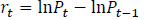is the log-return of a sample of equity prices. Now the ACD model is an extension of the GARCH with additional parameters specified to capture time-varying third and fourth moments of the distribution as:

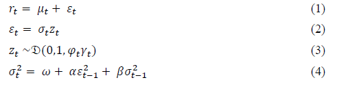
With the usual parameter constraints on to ensure the positivity of the variance.

The innovations driving the randomness are drawn from a distribution with the additional parameters and which have been parameterized as:

and

respectively.

The skew parameter describes the departure of the distribution from symmetry while the shape parameter controls the kurtosis of the tails. Both are used in calculating the respective time-varying third and fourth moments of the distribution. are transformation functions which ensure that the motion dynamics of the parameters are bounded in the interval of the real line.L and U are chosen to reflect the region of interest for .

For purposes of analysis, Hansen (1994) and Jondeau and Rockinger (2003), provided descriptions of the motion dynamics parametrized for the skew and kurtosis respectively as

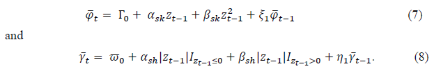
The coefficientsrepresent the forcing parameters driving the motion dynamics of the differential equations (5) and (6) respectively. are the regression constants, and represent the model coefficients with denoting respectively the skew and shape.

Parameter Estimation and Inference

Following the notation of Hansen (1994), the log-likelihood for the conditional functions can be written as:

With the vector as the parameter space containing the descriptors of the distribution and

inding the maximum likelihood estimate, involves writing the optimizations conditions

and solving for .

The s obtained from the above are point estimates with a lot of uncertainty. We estimate the uncertainty around these estimates using robust errors first suggested by White (1982). The variance-covariance of the square error matrix is given by:

where

and

The square roots of the leading diagonal of this matrix constitute the robust errors associated with our estimates.

Data Description and Analysis

We used a sample of daily aggregate index levels of the JSE-ASI from January 02, 2003 to December 31, 2017. The plot of the evolution of the index over the period is shown in Figure 1.

Figure 1 shows that the level of the JSE ALSI is gyrating over time but overall it is trending upwards. The market index took a tumble during 2007-2009, a period coinciding with the global financial crisis. The first difference of the logs of prices was analysed to get the returns which are presented in Figure 2.

It can be seen in Figure 2 that the returns across the period have been generally turbulent, particularly, during the years 2007-2009 when volatility was extremely high. Volatility clusters can be seen as characterising the evolutions of returns in the sample period.

We conducted unit root test to assess stationarity of the returns series using the Augmented Dickey-Fuller test. The test returned a with a p-value =0.01;hence we reject non-stationarity and conclude the series is stationary. The basic statistics of the data is summarised in Table 1.

Table 1: Summary Statistics
No. of Obs	Min	Max	1st Quartile	Median	3rd Quartile	Variance	Skewness	Ex Kurtosis
3748	-7.3824	6.8772	-0.5571	0.0927	0.7195	1.3986	-0.1669	3.6724

We plotted the histogram of the returns in the left of Figure 3 and overlapped it with the normal distributed curve. Clearly there is a marked departure from normality as confirmed by the excess kurtosis in Table 1. There is also slight negative asymmetry.

Again, the marked departure from normality is confirmed by the quantile-quantile plot on the right of Figure 3 showing clearly the deviation from the Gaussian distribution at the tails. A formal Cramer-von Mises test was carried out for normality. This generated a p-value of confirming the log-returns are not normal. This provides the reason to seek the descriptors of the higher moments.

The presence of (G)ARCH effects was investigated using Engle's LM test. The test returned a with a p-value confirming the presence of G(ARCH) effects. We fit the GARCH(1,1)-ACD-NIG models to the data with the racd package developed by Ghalanos (2016) using the R language (R Core Team, 2018). Table 2 displays the results of the ACD model from the analysis.

Table 2: Parameter Estimates Of Acd Model
	Estimate	Std. Error	t- value	p-value
	0.000789	0.00013	6.0811	0.0000
AR(1)	0.876772	0.020183	43.44063	0.0000
MA(1)	-0.90846	0.015847	-57.3281	0.0000
	0.083218	0.00172	48.37585	0.0000
	0.906974	0.000128	7072.701	0.0000
	-0.30709	1.040746	-0.29506	0.7679
	-0.0136	0.097237	-0.13988	0.8888
	0.541614	1.5493	0.34959	0.7266
	0.428893	0.478971	0.89545	0.3705
	0.112914	0.14912	0.7572	0.4489
	0.664015	0.154398	4.30066	0.0000
	0.008002	0.61173	0.01308	0.9896
	0.000001	NA	NA	NA

*Prefix: sk stands for skew and sh stands for shape

It can be inferred from Table 2 that the parameter of the higher fourth moment, is significant with a low p-value. This parameter determines the kurtosis of the distribution of returns. Thus, tail events will be dominant in the market. The result is consistent with the summary statistics in Table 1 which shows a slight left skew but an elevated kurtosis. Returns are, on the average, evenly distributed around the mean for the sample period.

Table 3 compares the various information criteria for the respective models ACD and GARCH. The Akaike, Shibata and Hannan-Quinn information criteria selected the ACD models as providing a better model fit to the data. As a rule, the Bayes criterion penalizes heavily complex models which the ACD is in an attempt to capture higher moment dynamics. Therefore, we can conclude that the finding is consistent.

Table 3: Information Criteria Of Models
	ACD	GARCH
Akaike	-6.3554	-6.3518
Bayes	-6.3355	-6.3418
Shibata	-6.3555	-6.3518
Hannan-Quinn	-6.3483	-6.3482

The evolution of the conditional volatility during the sample period is shown in Figure 4, which shows that risk pressures were dominant in the period leading up to the global financial crisis in 2008-2009. Volatility was highest during the financial crisis showing the contagious effects from the developed markets. Volatility has remained at pre-crisis levels since then with occasional flare ups due to developments in the underlying economy.

As Figure 5 shows, the skew varies wildly occasionally, however. Investor strategies and appetite for risk will determine where to ignore this fluctuations in skew or to keep an eyes on it.

On the other hand, the shape of the distribution is significant. There is a higher probability of extreme outcomes than specified by a normal distribution of returns. This, investors cannot ignore.

Figure 6 shows the varying nature of the fourth moment of the distribution of returns. The graph shows kurtosis does rise to extremes during market trading rather very often. The effect of fat-tails on asset allocations to risk management decisions is well documented in finance literature (Christoffersen & Diebold, 2000; Rosenberg & Schuermann, 2006). Tail events arising out of fat-tails have sparked financial crises so often over the past three decades that modelling the risk of tails of financial returns has spawned a whole new research stream in finance. Jorion (2000) attributed the demise of Long-Term Capital Management to being caught out by tail events. These tail events, according to Hartmann, Straetmans and Vries (2004), tend to be more severe when markets are in turmoil. This has been confirmed in a recent study of the effect of tail risk on asset prices by Kelly and Jiang (2014).

This study investigated the coverage levels by backtesting both the ACD and GARCH models at 1% and 5% respectively to ascertain the soundness of these models in estimating firm risk exposures. We relied on the Christoffersen's (1998) joint test for independence and correct coverage using the conditional coverage test. This test requires that the violations or VaR exceedances do not exceed given expected levels and also that they be conditionally independent. Table 4 presents the results with the plots at the respective 1% and 5% exhibited in Figure 7.

Table 4: Coverage Test Results For Acd And Garch At 1% And 5%
	expected.exceedances	actual.exceedances	cc.LRp	cc.Decision
ACD(1%)	17	20	0.666	Fail to Reject H0
ACD(5%)	87	87	0.946	Fail to Reject H0
GARCH(1%)	17	18	0.823	Fail to Reject H0
GARCH(5%)	87	90	0.946	Fail to Reject H0

Results show that our analysis generated the correct number of VaR exceedances which are independent too as shown by the likelihood ratio for the conditional coverage (cc.LRp) column; hence we fail to reject either of the models. In either case, at the 1% coverage level, the GARCH model performs better as a risk model than the ACD model. However, at 5% coverage level, the test is unable to discriminate among the models. Lastly, we tested for the goodness of fit of the tail distribution using the Berkowitz test (Berkowitz, 2001), testing at the 1% quantile. Both models generated higher p-values with the GARCH model seemingly slightly providing a better fit in the tails. This anomaly, even though not severe, should be investigated further. Overall looking at the exhibit in Table 5, we fail to reject the null hypothesis that the ACD and GARCH models properly fit the tails of the distribution.

Table 5: Results Of Good-Of-Fit Using Berkowitz Test
	uLL	rLL	LRp	Decision
ACD	-108.46	-108.66	0.8191	Fail to reject H0
GARCH	-99.59	-99.61	0.9802	Fail to reject H0

The test results both from Tables 4 and 5 suggest that the GARCH model provide overall model fit compared to the ACD model. However, Hwang and Satchell (1999) stress the important of higher moments in properly estimating market risk in emerging markets. This point is further buttressed by Harvey (2000), who claims that the second moment is not enough in characterising risks in international markets outside the US. This would suggest there are lurking risks in the higher moments that investors must consider.

Conclusion

Emerging market assets can look cheap if they are not properly priced. This could be the result of under estimation of risk leading to such mispricing. Describing the distribution of market returns by variance alone is based on assumptions that cannot be defended in the face of empirical observation of return distributions. By capturing time-varying skew and shape of the returns, ACD models provide a complete description of the risk spectrum of the market returns. The ACD models situate volatility estimation within the experiences of market practitioners largely from first principles. GARCH models do not tell the whole story of volatility of market returns.

The deficiencies in the current generation of risk models have been highlighted extensively by Jorion (2009), Danielsson (2008), Sarma, Thomas and Shah (2003) and Eberlein, Keller and Prause (1998), among others. For long GARCH models and their variants have been the mainstay in finance for volatility modelling. But as shown by Danielsson and de Vries (2000), such models are unsuitable to calculating risk on a large scale. ACD models provide a better fit for the returns of equities as long as they capture the full range of moments that describe the fully the distribution of returns.

Aloui et al. (2011) posit that fat-tails are increasingly observed in equity returns coming from emerging markets of which includes the Johannesburg Stock Exchange. Thus, investors can no longer ignore these dimensions of risk. Fat-tails add to the risk of returns from equities on the JSE and this should be recognized by market actors. In the extreme cases, the left tails of distributions of returns from the aggregate index of the JSE should be isolated and analyzed to reveal the hidden risks likely to spring surprises on investors. Indeed, this is the recommendation of Mittnik, Paolella and Rachev (2000). This should be even more relevant today given the frequency of market turmoil.

Our study provides evidence that higher moments, especially the fourth moment, are needed to completely describe the risk of market returns during the sample period. However, goodness-of-fit tests could not discriminate clearly between traditional GARCH (1,1) model on the one hand and the GARCH(1, 1)-ACD-NIG model on the other hand. We think this is due to using an aggregate market index which confers properties different those of the constituent stocks on the data. We think this work needs further investigation using the individual stocks constituting the broad JSE market index.

References

1. Aloui, R., Aïssa, M.S., & Nguyen, D.K. (2011). Global financial crisis, extreme interdependences, and contagion effects: The role of economic structure? Journal of Banking & Finance, 35(1), 130-141.
2. Anderson, R.W., & Harris, C.J. (1986). A model of innovation with application to new financial products. Oxford Economic Papers, 38, 203-218.
3. Babikir, A., Gupta, R., Mwabutwa, C., & Owusu-Sekyere, E. (2012). Structural breaks and GARCH models of stock return volatility: The case of South Africa. Economic Modelling, 29(6), 2435-2443.
4. Barroso, P., & Santa-Clara, P. (2015). Momentum has its moments. Journal of Financial Economics, 116(1), 111-120.
5. Berkowitz, J. (2001). Testing density forecasts, with applications to risk management. Journal of Business & Economic Statistics, 19(4), 465-474.
6. Bollerslev, T. (1986). Generalized autoregressive conditional heteroskedasticity. Journal of econometrics, 31(3), 307-327.
7. Britten-Jones, M., & Schaefer, S. M. (1999). Non-linear value-at-risk. Review of Finance, 2(2), 161-187.
8. Chinzara, Z. (2011). Macroeconomic uncertainty and conditional stock market volatility in South Africa. South African Journal of Economics, 79(1), 27-49.
9. Christoffersen, P.F. (1998). Evaluating interval forecasts. International Economic Review, 841-862.
10. Christoffersen, P.F., & Diebold, F.X. (2000). How relevant is volatility forecasting for financial risk management? Review of Economics and Statistics, 82(1), 12-22.
11. Coles, S. (2001). An Introduction to Statistical Modeling of Extreme Values. New York: Springer-Verlag.
12. Cont, R. (2001). Empirical properties of asset returns: stylized facts and statistical issues. Quantitative Finance, 1(2), 223-236.
13. Danielsson, J. (2008). Blame the models. Journal of Financial Stability, 4(4), 321-328.
14. Danielsson, J., & De Vries, C.G. (2000). Value-at-risk and extreme returns. Annales d'Economie et de Statistique, 239-270.
15. Eberlein, E., Keller, U., & Prause, K. (1998). New insights into smile, mispricing, and value at risk: The hyperbolic model. The Journal of Business, 71(3), 371-405.
16. Engle, R.F. (1982). Autoregressive conditional heteroscedasticity with estimates of the variance of United Kingdom inflation. Econometrica: Journal of the Econometric Society, 987-1007.
17. Engle, R.F., & Bollerslev, T. (1986). Modelling the persistence of conditional variances. Econometric Reviews, 5(1), 1-50.
18. Engle, R.F., & Gonzalez-Rivera, G. (1991). Semiparametric ARCH models. Journal of Business & Economic Statistics, 9(4), 345-359.
19. Fang, H., & Lai, T.Y. (1997). Co?kurtosis and capital asset pricing. Financial Review, 32(2), 293-307.
20. Gencay, R., & Selcuk, F. (2004). Extreme value theory and value-at-risk: Relative performance in emerging markets. International Journal of Forecasting, 20(2), 287-303.
21. Ghalanos, A. (2016). racd: Autoregressive Conditional Density Models. https://bitbucket.org/alexiosg/.
22. Guidolin, M., & Timmermann, A. (2008). International asset allocation under regime switching, skew, and kurtosis preferences. The Review of Financial Studies, 21(2), 889-935.
23. Hansen, B.E. (1994). Autoregressive conditional density estimation. International Economic Review, 705-730.
24. Hartmann, P., Straetmans, S., & Vries, C.D. (2004). Asset market linkages in crisis periods. Review of Economics and Statistics, 86(1), 313-326.
25. Hartz, C., Mittnik, S., & Paolella, M. (2006). Accurate value-at-risk forecasting based on the normal-GARCH model. Computational Statistics & Data Analysis, 51(4), 2295-2312.
26. Harvey, C.R. (2000). The Drivers of Expected Returns in International Markets. Durham, NC, USA. doi:http://dx.doi.org/10.2139/ssrn.795385
27. Harvey, C.R., & Siddique, A. (2000). Conditional skewness in asset pricing tests. The Journal of Finance, 55(3), 1263-1295.
28. Hwang, S., & Satchell, S.E. (1999). Modelling emerging market risk premia using higher moments. International Journal of Finance & Economics, 4(4), 271-296.
29. Jondeau, E., & Rockinger, M. (2003). Testing for differences in the tails of stock-market returns. Journal of Empirical Finance, 10(5), 559-581.
30. Jondeau, E., & Rockinger, M. (2012). On the importance of time variability in higher moments for asset allocation. Journal of Financial Econometrics, 10(1), 84-123.
31. Jorion, P. (2000). Risk management lessons from long?term capital management. European Financial Management, 6(3), 277-300.
32. Jorion, P. (2009). Risk management lessons from the credit crisis. European Financial Management, 15(5), 923-933.
33. Kelly, B., & Jiang, H. (2014). Tail risk and asset prices. The Review of Financial Studies, 27(10), 2841-2871.
34. Kim, Y.S., Rachev, S.T., Bianchi, M.L., Mitov, I., & Fabozzi, F.J. (2011). Time series analysis for financial market meltdowns. Journal of Banking & Finance, 35(8), 1879-1891.
35. Kratz, O.S. (1999). The Philology of Frontier Equity Markets. In Frontier Emerging Equity Markets Securities Price Behavior and Valuation (pp. 179-190). Boston, MA: Springer.
36. Liu, S.M., & Brorsen, B. (1992). Maximum Likelihood Estimation of the Stable Distribution with a Time-Varying Scale Parameter. Unpublished Working Paper. Purdue University.
37. Longin, F. (1996). The asymptotic distribution of extreme stock market returns. Journal of Business, 69, 383-408.
38. Markowitz, H. (1952). Portfolio selection. The Journal of Finance, 7(1), 77-91.
39. McMillan, D., & Thupayagale, P. (2010). Evaluating stock index return value-at-risk estimates in South Africa: Comparative evidence for symmetric, asymmetric and long memory GARCH models. Journal of Emerging Market Finance, 9(3), 325-345.
40. McNeil, A.J., & Frey, R. (2000). Estimation of tail-related risk measures for heteroscedastic financial time series: an extreme value approach. Journal of Empirical Finance, 7(3-4), 271-300.
41. Mittnik, S., Paolella, M.S., & Rachev, S.T. (2000). Diagnosing and treating the fat tails in financial returns data. Journal of Empirical Finance, 7(3-4), 389-416.
42. Muela, S.B., Martín, C.L., & Sanz, R.A. (2017). An application of extreme value theory in estimating liquidity risk. European Research on Management and Business Economics, 23(3), 157-164.
43. Oberholzer, N., & Venter, P. (2015). Univariate GARCH models applied to the JSE/FTSE stock indices. Procedia Economics and Finance, 24, 491-500.
44. Perez-Quiros, G., & Timmermann, A. (2001). Business cycle asymmetries in stock returns: Evidence from higher order moments and conditional densities. Journal of Econometrics, 103(1-2), 259-306.
45. Poon, S.H., Rockinger, M., & Tawn, J. (2003). Extreme value dependence in financial markets: Diagnostics, models, and financial implications. The Review of Financial Studies, 17(2), 581-610.
46. R Core Team. (2018). R: A language and environment for statistical computing. R Foundation for Statistical Computing. Vienna. Retrieved from https://www.R-project.org/
47. Rosenberg, J.V., & Schuermann, T. (2006). A general approach to integrated risk management with skewed, fat-tailed risks. Journal of Financial Economics, 79(3), 569-614.
48. Sarma, M., Thomas, S., & Shah, A. (2003). Selection of Value?at?Risk models. Journal of Forecasting, 22(4), 337-358.
49. Singh, A.K., Allen, D.E., & Robert, P.J. (2013). Extreme market risk and extreme value theory. Mathematics and computers in simulation, 94, 310-328.
50. Szegö, G. (2002). Measures of risk. Journal of Banking & Finance, 26(7), 1253-1272.
51. Uppal, J.Y., & Ullah Mangla, I.U. (2013). Extreme loss risk in financial turbulence-evidence from the global financial crisis. Managerial Finance, 39(7), 653-666.
52. White, H. (1982). Maximum likelihood estimation of misspecified models. Econometrica: Journal of the Econometric Society, , 1-25.
53. Wilhelmsson, A. (2009). Value at Risk with time varying variance, skewness and kurtosis-the NIG?ACD model. The Econometrics Journal, 12(1), 82-104.