Introduction

Uncertainty — commonly referred to as volatility — plays a crucial role in financial theories. Many models in finance use the variance (or standard deviation) as a measure of uncertainty. In most of these models, the variance is assumed to be homoscedastic, meaning that it is constant through time. However, empirical evidence on financial time series data has disproved this assumption. It has been established that the volatility of financial time series exhibits stylised empirical facts such as non-Gaussian distributions (characterised by excess kurtosis), fat-tailed distributions (characterised by the law of decay in the tail of the distribution), high-frequency persistence (characterised by super-diffusive behaviour at short time scales), volatility clustering (characterised by non-stationarity in price changes), and leverage effect (where negative returns tend to increase the volatility by more significant amounts than positive returns of the same magnitude) (Jiang et al., 2019).

Not only volatility in financial time series persist over a while (that is, high returns follow high volatility and low returns follow low volatility), giving rise to volatility clustering discussed above, but it can also spread from one market to another, resulting in what is termed volatility spillover (Patnaik, 2013). Volatility spillovers have been identified in the academic financial literature “as the cause and/or effect of financial contagion” (Roy & Roy, 2017:1), consequently, in studies such as Abou-Zaid (2011) and Diebold & Yilmaz (2008), the terms volatility spillover and contagion interchangeably. In its pure form¹, financial contagion refers to the propagations of shocks due to reasons that are not related to shocks in macroeconomic fundamentals. The propagations are solely the result of irrational phenomena, such as panics, herd behaviour, loss of confidence and risk aversion. In this context financial contagion is characterised by an increase in cross-market correlations during crisis periods, relative to correlations during tranquil periods

Financial contagion has been viewed primarily as concern for emerging markets (Aderajo & Olaniran, 2021). Kaminsk, Reinhar and  Végh (2003) identified three key elements, which they dubbed the “unholy trinity”, that make emerging markets prone to contagions; they are, (i) an abrupt reversal in capital inflow, (ii) a surprise announcement, and (iii) a leveraged common creditor. Regarding the reversal in capital inflow Kaminsk, Reinhar and Végh (2003) noted that before financial contagions, crisis-prone markets experience a surge in international capital inflow, but after the initial shock has taken place, the affected economies experience an abrupt halt in capital inflow. Regarding surprise announcements, they explained that an unexpected announcement triggers a chain reaction that always comes as a surprise to the financial market. Regarding a common creditor, Kaminsk, Reinhar and Végh (2003) stressed that in most cases a leveraged common creditor is involved, as is the case for American banks in Latin American crises or Japanese banks in Asian crises.

This article investigates financial contagion in BRICS equity market by analysing volatility spillover and time-varying correlations in BRICS stock markets in the wake of the U.S. sub-prime and Eurozone sovereign debt crises. The article uses a Multivariate Autoregressive Conditional Heteroskedasticity (MGARCH) model as a measure of volatility spillover. Identifying volatility spillover and time-varying correlations byways of multivariate modelling results in more insightful analysis than operating with separate univariate models. From a financial perspective, it paves the way to better decision-making tools in different fields, such as asset pricing, portfolio selection, option pricing, hedging, and risk management (Malumisa, 2015).

The rest of this article is structured as follows. Section two presents the time series data used in the current study. The section also discusses the empirical models and the estimation methodology used. The empirical results obtained from the analysis are presented in section three. The section four concludes with a summary and section five discusses policy recommendations.

Data and Methodology

This section describes the data and econometric model used to investigate financial contagion in BRICS stock market following the sub-prime crisis which emanated from the U.S and the EZDC that emanated from Eurozone countries. The econometric model used is the Dynamic Conditional Correlation (DCC)-GARCH. 

Data

The data used in the present study comprise daily closing stock price of indices from individual BRICS countries, Germany and the United States. The data spans a period between 11^th of January 2005 and 26^th of December 2017 (providing 2443 daily observations for each market). The ‘target’ stock market indices examined consist of those in the Brazilian BOVESPA (São Paulo Stock Exchange/Bolsa de Valores de São Paulo index), the Chinese SSE (Shanghai Stock Exchange index,), the Indian SENSEX (Bombay Stock exchange index), the Russian RTS (Moscow Exchange index) and the South African FTSE/JSE All share (Johannesburg Stock Exchange index, hereafter referred as FTSE/JSE). While ‘source’ (ground zero) markets are the daily stock price index of the United States, the S&P 500, and the German, DAX Composite index is used as the proxy for the Eurozone (continental Europe) stock market. Figures 1-2 displays the time series plot of indices used in the current study. The time series is non-stationary due to the non-constant mean.

For detrending, and in order to achieve more stationary time series data, the daily price indices were transformed into natural logarithmic returns expressed as follows:

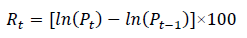
where P_t is the closing price index recorded for period t , and P_t-1 is the closing price index recorded for period t-1. The reason for multiplying the expression ln (P_t) − ln (P_t-1) by 100 is due to numerical problems in the estimation part. This will not affect the structure of the model since it is just a linear scaling.

For each of the two crises that were examined for potential financial contagion (i.e. sub-prime and EZDC), the set of data used were divided into two sub-periods, (i) the turbulent period and (ii) the stable period. For instance, in order to examine financial contagion in BRICS equity markets following the sub-prime crisis, this article uses two sub-periods, they are the (i)‘pre-crisis’(Panel A) sub-period that ranges from 11^th February 2005 to  1^st February 2007 and (ii) the ‘crisis’ (Panel B) sub-period that extends from  2^nd February 2007, — the date that corresponds with the explosion of the real estate bubble in the U.S. — to  10^th July 2009. In order to analyse volatility spillover in BRICS equity markets emanating from the Eurozone, the current study uses two sub-periods: they are (i) the ‘crisis’ (Panel C) sub-period which spans from 12^th August 2009 — the date that matches the Greek government defaulting on its debt — to 31^st December 2012, and (ii) the ‘post-crisis’ (Panel D) sub-period that starts on 1^st January 2013 and ends on 28^th February 2017 in the aftermath of the Eurozone sovereign debt crisis. While for the sub-prime crisis we use a crisis and a pre-crisis period, the authors are of the opinion that the period prior to the Eurozone crisis was also characterised by financial turmoil and is thus not a good representation of a tranquil period.

Methodology            

The Dynamic Conditional Correlation (DCC)-GARCH model introduced by Engle (2002) was used to examine volatility spillover in BRICS stock markets following the financial crises that took place in the U.S. and Eurozone countries. The DCC-GARCH model is a dynamic model with time-varying mean, variance and covariance of return series r_t with the following mean equation:

r_t = u_t+ε_t .………………………………………………........(1)

           

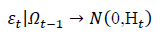
From the residuals of the equation 1, the conditional variance of each return is derived using Equation 2 given below.

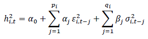……….…………. (2)

Then the multivariate conditional variance H_t is estimated as follows:

H_t= D_tR_tD_t…………. (3)

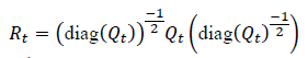
where H_t is the Conditional Covariance matrix of r_t , D_t represents a (k × k) diagonal matrix of time-varying standard deviations obtained from the univariate GARCH specifications given in Equation 2, R_t is the (k x k) time-varying correlations matrix derived by first standardising the residuals of the mean Equation 1 of the univariate GARCH model with their conditional standard deviations derived from Equation 2, to obtain .

The standardised residuals are then used to estimate the parameters of conditional correlation as given in equation 4 and 5 below.

…………. (4)

and

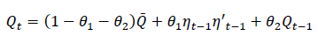…………(5)

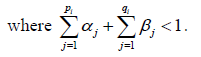
where  is the unconditional covariance of the standardised residuals. The Q_t does not generally have ones on the diagonal, so it is scaled as in Equation 4 above to derive R_t ,which is a positive definite matrix. In this model, the conditional correlations are thus dynamic, or time-varying. θ₁ and θ₂  from Equation 5 are assumed to be positive scalars with θ₁ + θ₂ < 1.

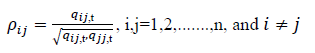
Finally, the conditional correlation coefficient, , between two market returns, i and j, is expressed by the following equation:

……………………(6)

and can be expressed in typical correlation form by putting Q_t = q_{i j,t} as follows:

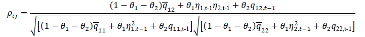………………………(7)

The parameters of the DCC model are estimated using the likelihood for this estimator and can be written as:

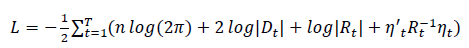………………….….(8)

Where 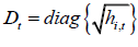and R_t is the time-varying correlation matrix.

As mentioned in section 1, the stylised facts of financial time series data deviate in two respects from the usual white noise generated from a Gaussian stochastic process. Firstly, the unconditional distribution is severely leptokurtic. In other words, it is more peaked in the centre and displays fat tails, with more unusually large and small observations than would be implied from the Gaussian law. Secondly, they exhibit volatility clustering, where calm and volatile episodes are observed, such that at least the variance appears to be predictable (Chinzara & Azakpioko, 2009). Consequently, Gaussian assumptions in the DCC-GARCH procedure can be violated. To circumvent this problem, the t-DCC-GARCH procedure is used in which the DCC model is applied with an assumption that market yields follow a multivariate t-distribution as suggested by (Pesaran & Pesaran, 2007). To achieve this, Pesaran & Pesaran (2007) introduced the use of devolatilised returns which are approximately Gaussian, instead of standardised returns. The devolatilised returns   are computed by allowing returns to be normalised by realised volatility rather than by conditional volatilities in the GARCH-type models (Barassi et al., 2011).

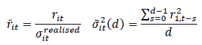……………. (9)

The devolatilised returns,   are used in Equation 2 to calculate the conditional correlations.

It is worth noting that the current study uses univariate GARCH (1,1) process is used hence the equation becomes

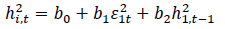  ………….…………(10)

Results of Empirical Models and Discussion

This section uses bivariate GARCH models to examine volatility spillover in BRICS, as ‘target’ market², from ‘source’ markets, namely U.S. and Eurozone stock markets.

Estimations of DCC Garch Model

This section provides the estimation results for the mean, variance, and correlation model using the DCC GARCH model as introduced in the methodology section.

Estimations of DCC GARCH Model for Financial Contagion Following the Sub-prime Crisis

In order to examine financial contagion in BRICS stock markets following the sub-prime crisis in the US, the present study estimates the following coefficients: (i) the mean (Equation 1), (ii) the variance (Equation 2), and (iii) the correlation model (Equation 7) using the DCC GARCH model. The coefficient was estimated for both the ‘pre-crisis’ and ‘crisis’ periods. The results for bivariate estimations of the DCC GARCH model between the S&P500 and individual BRICS stock markets indices are presented in Tables 1 to 5.

Table 1 Estimation Parameters of Mean, Variance, and Correlation Models of Contagion with the U.S. as Source Country and Brazil as Target Country
	Parameter	Pre-crisis			crisis
		Estimate	SE	P-value	Estimate	SE	P-value
S&P500	α0	0.030612	0.015175	0.043664	0.026354	0.019309	0.172304
	α1	0.088054	0.040294	0.028869	0.098974	0.021360	0.000004
	β1	0.834843	0.053447	0.000000	0.896712	0.019533	0.000000
BOVESPA	α0	0.113157	0.120138	0.346246	0.112314	0.073492	0.126450
	α1	0.079405	0.051562	0.123563	0.084119	0.024557	0.000614
	β1	0.875195	0.079141	0.000000	0.893265	0.027903	0.000000
	θ1	0.048020	0.016823	0.004312	0.046595	0.013976	0.000856
	θ2	0.939771	0.023229	0.000000	0.947932	0.016114	0.000000
ρij[corr(S&P500,BOVESPA)]				0.6150935	ρij[ corr(S&P500,BOVESPA)]		0.7678467
Maximized Log-likelihood				-889.6288	Maximized Log-likelihood		-1617.114

Table 2 Estimation Parameters of Mean, Variance, and Correlation Models with the U.S. as Source Country and South Africa as Target Country
		Pre-crisis				Crisis
	Parameter	Estimate	SE		P-value	Estimate	SE	P-value
S&P500	α0	0.030612	0.015351		0.046139	0.026354	0.018993	0.165272
	α1	0.088054	0.040324		0.028986	0.098974	0.021543	0.000004
	β1	0.834843	0.053720		0.000000	0.896712	0.019551	0.000000
FTSE/JSE	α0	0.034016	0.021301		0.110281	0.058724	0.030377	0.053210
	α1	0.165848	0.048839		0.000684	0.112168	0.025988	0.000016
	β1	0.819095	0.045508		0.000000	0.869951	0.025714	0.000000
	θ1	0.004620	0.012811		0.718359	0.001380	0.020384	0.946037
	θ2	0.968608	0.029602		0.000000	0.887137	0.887137	0.004369
ρij[ corr(S&P500,JSE)]				0.2400472		ρij[corr(S&P500,JSE)]		0.4250802
Maximized Log-likelihood				-820.6837		Maximized Log-likelihood		-1655.506

Table 3 Estimation Parameters of Mean, Variance, and Correlation Model with the U.S. as Source Country and Russia as Target Country
		Pre-crisis			crisis
	Parameter	Estimate	SE	P-value	Estimate	SE	P-value
S&P500	α0	0.030612	0.015287	0.045227	0.026354	0.019068	0.166942
	α1	0.088054	0.040460	0.029530	0.098974	0.021298	0.000003
	β1	0.834843	0.053555	0.000000	0.896712	0.019442	0.000000
RTS	α0	0.114489	0.067514	0.089928	0.078782	0.047885	0.099921
	α1	0.125094	0.048935	0.010579	0.117498	0.034544	0.000670
	β1	0.835400	0.050359	0.000000	0.875790	0.027331	0.000000
	θ1	0.005913	0.012067	0.624097	0.038157	0.046055	0.407381
	θ2	0.968719	0.021778	0.000000	0.815539	0.250268	0.001119
ρij[ corr(S&P500,RTS)]				0.1464534	ρij[ corr(S&P500,RTS)]		0.3306286
Maximized Log-likelihood				-959.4556	Maximized Log-likelihood		-1839.87

Table 4 Estimation Parameters of Mean, Variance, and Correlation Model with the U.S. as Source Country and India as Target Country
		Pre-crisis			crisis
	Parameter	Estimate	SE	P-value	Estimate	SE	P-value
S&P500	α0	0.030612	0.015344	0.046038	0.026354	0.019037	0.166241
	α1	0.088054	0.040432	0.029416	0.098974	0.021347	000004
	β1	0.834843	0.053672	0.000000	0.896712	0.019541	0.000000
SENSEX	α0	0.151964	0.064974	0.019343	0.152778	0.130993	0.243491
	α1	0.154722	0.053949	0.004132	0.145174	0.049816	0.003566
	β1	0.755650	0.069218	0.000000	0.842642	0.052391	0.000000
	θ1	0.000000	0.000029	0.999115	0.040532	0.028250	0.151350
	θ2	0.919327	0.178326	0.000000	0.850395	0.064644	0.000000
ρij[ corr(S&P500,SENSEX)]				0.152096	ρij[ corr(S&P500,SENSEX)]		0.280337
Maximized Log-likelihood				-902.7562	Maximized Log-likelihood		-1818.645

Table 5 Estimation Parameters of Mean, Variance, and Correlation Model with the U.S. as Source Country and China as Target Country
		Pre-crisis			crisis
	Parameter	Estimate	SE	P-value	Estimate	SE	P-value
S&P500	α0	0.030612	0.015344	0.046039	0.026354	0.019025	0.165987
	α1	0.088054	0.040432	0.029417	0.098974	0.021456	0.000004
	β1	0.834843	0.053672	0.000000	0.896712	0.019549	0.000000
SSE	α0	0.085463	0.057525	0.137367	0.187103	0.155137	0.227796
	α1	0.041964	0.027015	0.120334	0.079929	0.032844	0.014949
	β1	0.918015	0.029109	0.000000	0.893193	0.035316	0.000000
	θ1	0.000000	0.000158	0.999965	0.011784	0.016465	0.474168
	θ2	0.919882	0.593842	0.121373	0.964742	0.040455	0.000000
ρij[ corr(S&P500,SSE)]				0.0234467	ρij[ corr(S&P500,SSE)]		0.03179588
Maximized Log-likelihood				-947.4045	Maximized Log-likelihood		-1887.203

The results present a summary of the DCC model parameter estimates for both the ‘pre-crisis’ and the ‘crisis’ periods. Each table presents source-target pairs consisting of the U.S. and an individual BRICS market. Most of the parameter estimates for univariate GARCH (1,1) as represented in the diagonal elements of Dt in Equation 3 and 5 appear to be signi?cantly di?erent from zero at the 10% level of signi?cance. This means that, following the sub-prime crisis in the US, equity markets in BRICS countries reacted to shocks emanating from the U.S. equity market, in both the ‘pre-crisis’ and ‘crisis’ periods

The significant coefficients α1 for most stock markets (except for China) are indicating the persistence of volatility which suggests possible transmissions of volatility from the U.S. stock market. The coefficient β1 is also significant in most markets and indicates a large asymmetric impact, implying that BRICS stock markets are reacting to different sources of information from different markets and consequently adapting their portfolios. The DCC-GARCH (1, 1) parameters θ₁ and θ₂ are also presented in Tables 1 through Table 5. The parameters measure the impact of past standardised shocks (θ₁) and lagged dynamic conditional correlations (θ₂) on the current dynamic conditional correlations. The tables suggest that only θ₂ is significant in most BRICS equity markets, implying that lagged dynamic conditional correlations is the only one that has significant effects (except for China). Joint significance parameters θ₁ and θ₂ is only found in the Brazilian stock market. (Joint significance means that the DCC model is adequate at measuring in time-varying conditional correlations). The necessary condition of θ₁ + θ₂ < 1 holds for all pairwise indices. It is worth noting that the mean value of the conditional correlation coefficient (ρ_ij) across pairs of stock market is of a higher magnitude in the ‘crisis’ period that the ‘pre-crisis’ period.

A plot of the estimated conditional correlations using the DCC model is presented in Figures 2 to 6. The general impression of the conditional correlations increased significantly during the ‘crisis’ period as compared to the ‘pre-crisis’ period. The conditional correlation reached its highest level towards the end of the year 2008, which corresponds with the bankruptcy filing of Lehman Brothers on September 15^th 2008. Lehman Brothers was one of the oldest and largest investment banking firms in the world, and its collapse deepened the then -ongoing U.S. financial crisis.

Given the fact that conditional correlation coefficients increased considerably during the sub-prime crisis, — except for China (SSE) and Indian (SENSEX) —is an indication that financial contagion emanating from the U.S. took place in BRICS stock markets. For the Chinese market, the lack of contagion might be because strong government control of the Chinese stock market insulated the Chinese equity market from contagious effects from the US. Furthermore, as Naoui et al. (2010) suggested, the decoupling of the Chinese market from financially contagious effects from the U.S. market can also be attributed to China’s growing economic strength at the time of financial contagion.

Estimations of DCC Garch Model for Financial Contagion Following the Eurozone Crisis

In order to examine financial contagion in BRICS stock markets following the Eurozone sovereign debt crisis in the Eurozone countries, the current study estimates coefficients for the mean (Equation 1), the variance (Equation 2) and correlation models (Equation 7) using the DCC GARCH model. The coefficient was estimated for both the ‘crisis’ and ‘post-crisis’ periods. The results for bivariate estimation between the DAX and individual BRICS stock market indices are presented in Tables 6 to 10.

Table 5 Estimation Parameters of Mean, Variance, and Correlation Model with the U.S. as Source Country and China as Target Country
		Pre-crisis			crisis
	Parameter	Estimate	SE	P-value	Estimate	SE	P-value
S&P500	α0	0.030612	0.015344	0.046039	0.026354	0.019025	0.165987
	α1	0.088054	0.040432	0.029417	0.098974	0.021456	0.000004
	β1	0.834843	0.053672	0.000000	0.896712	0.019549	0.000000
SSE	α0	0.085463	0.057525	0.137367	0.187103	0.155137	0.227796
	α1	0.041964	0.027015	0.120334	0.079929	0.032844	0.014949
	β1	0.918015	0.029109	0.000000	0.893193	0.035316	0.000000
	θ1	0.000000	0.000158	0.999965	0.011784	0.016465	0.474168
	θ2	0.919882	0.593842	0.121373	0.964742	0.040455	0.000000
ρij[ corr(S&P500,SSE)]				0.0234467	ρij[ corr(S&P500,SSE)]		0.03179588
Maximized Log-likelihood				-947.4045	Maximized Log-likelihood		-1887.203

Tables 6 to 10 present a summary of the DCC model parameter estimates for both the ‘crisis’ and the ‘post-crisis’ periods. Each table presents source-target pairs consisting of the DAX composite index as a proxy of the Eurozone (continental Europe) stock markets, and individual indices from BRICS stock markets. Most of the parameter estimates for univariate GARCH (1,1), as represented in the diagonal elements of D_t in Equation 3 and 5, assppear to be signi?cantly di?erent from zero at the 10% level of signi?cance. This means that, following the sovereign debt crisis in the Eurozone countries, equity markets in BRICS countries reacted equally to shock emanating from European equity market, in both the ‘crisis’ and ‘post-crisis’ periods.          

The significant coefficient α1 for most stock markets (except China) are indicating the persistence of volatility, which suggests possible transmissions of volatility from the European stock markets. The coefficient β₁ is also significant in most markets and indicates a large asymmetric impact, implying that BRICS stock markets are reacting to different sources of information from different markets and consequently adapting their portfolio. The DCC-GARCH (1,1) parameters θ₁ and θ₂ are presented in Tables 6 to 10; they measure the impact of past standardised shocks (θ₁) and lagged dynamic conditional correlations (θ₂) on the current dynamic conditional correlations. As in the case of the sub-prime crisis, the tables suggest that only θ₂ is significant in most BRICS equity markets, implying that it is the only one that has significant effects (except for China). Joint significance parameters θ₁ and θ₂ are only found in the Indian and the South African stock markets in the ‘post-crisis’ period. This means that the DCC model is adequate in these two countries’ stock markets. It is worth noting that, unlike the case of the sub-prime crisis, there are no significant differences between the mean value of the conditional correlation coefficient (ρ_ij) in the ‘crisis’ period compared to the ‘post-crisis’ period.

Table 6  Estimation Parameters of Mean, Variance, and Correlation Models of Contagion with the Eurozone Countries as Source Country and Brazil as Target Country
	Parameter	crisis			Post-crisis
		Estimate	SE	P-value	Estimate	SE	P-value
DAX	α0	0.103449	0.055202	0.060928	0.043241	0.036482	0.235910
	α1	0.118185	0.041146	0.004074	0.120033	0.051285	0.019258
	β1	0.830373	0.055211	0.000000	0.857878	0.063436	0.000000
BOVESPA	α0	0.302310	0.134154	0.024230	0.100942	0.044255	0.022551
	α1	0.138640	0.053052	008968	0.069881	0.017837	0.000089
	β1	0.719771	0.093178	0.000000	0.887347	0.029099	0.000000
	θ1	0.007570	0.009694	0.434855	0.023470	0.020304	0.247730
	θ2	0.963034	0.044093	0.000000	0.809986	0.075054	0.000000
ρij[ corr(DAX,BOVESPA)]				0.5760211	ρij[ corr(DAX,BOVESPA)]		0.3483692
Maximized Log-likelihood				-1961.107	Maximized Log-likelihood		-2374.321

Table 7 Estimation Parameters of Mean, Variance, and Correlation Models of Contagion with the Eurozone Countries as Source Country and South Africa as Target Country
	Parameter	Pre-crisis			crisis
		Estimate	SE	P-value	Estimate	SE	P-value
DAX	α0	0.103449	0.055671	0.063139	0.043241	0.036419	0.235103
	α1	0.118185	0.041526	0.004426	0.120033	0.051302	0.019298
	β1	0.830373	0.055782	0.000000	0.857878	0.063353	0.000000
FTSE/JSE	α0	0.053062	0.026005	0.041308	0.065181	0.024784	0.008540
	α1	0.133186	0.033212	0.000061	0.120050	0.032494	0.000220
	β1	0.818599	0.042404	0.000000	0.815082	0.045588	0.000000
	θ1	0.022089	0.021456	0.303233	0.018138	2.63951	0.008303
	θ2	0.657200	0.162710	0.000054	0.886743	0.059042	0.000000
ρij[ corr(DAX,FTSE/JSE)]				0.708764	ρij[ corr(DAX,FTSE/JSE)]		0.6070643
Maximized Log-likelihood				-1651.724	Maximized Log-likelihood		-1941.868

Table 8 Estimation Parameters of Mean, Variance, and Correlation Models of Contagion with the Eurozone Countries as Source Country and Russia as Target Country
	Parameter	Pre-crisis			crisis
		Estimate	SE	P-value	Estimate	SE	P-value
DAX	α0	0.103449	0.055206	0.060948	0.043241	0.036727	0.239050
	α1	0.118185	0.041843	0.004736	0.120033	0.051705	0.020261
	β1	0.830373	0.055553	0.000000	0.857878	0.06390	0.000000
RTS	α0	0.181433	0.181433	0.079663	0.079575	0.042561	0.061526
	α1	0.102632	0.039802	0.009921	0.088485	0.026527	0.000851
	β1	0.848464	0.054126	0.000000	0.888743	0.031128	0.000000
	θ1	0.015472	0.014282	0.278659	0.034820	0.018758	0.063407
	θ2	0.952225	0.065886	0.000000	0.955482	0.034678	0.000000
ρij[ corr(DAX,RTS)]				0.6441123	ρij[ corr(DAX,RTS)]		0.5007368
Maximized Log-likelihood				-2061.619	Maximized Log-likelihood		-2415.707

Table 9 Estimation Parameters of Mean, Variance, and Correlation Models of Contagion with the Eurozone Countries as Source Country and India as Target Country
	Parameter	Pre-crisis			crisis
		Estimate	SE	P-value	Estimate	SE	P-value
DAX	α0	0.103449	0.055092	0.060415	0.043241	0.036404	0.234914
	α1	0.118185	0.040964	0.003913	0.120033	0.051374	0.019468
	β1	0.830373	0.055130	0.000000	0.857878	0.063402	0.000000
SENSEX	α0	0.030209	0.020288	0.136496	0.000851	0.005084	0.867025
	α1	0.060615	0.018185	0.000858	0.000000	0.005018	0.999784
	β1	0.918141	0.023983	0.000000	0.999000	0.000051	0.000000
	θ1	0.024007	0.014774	0.104172	0.018252	0.007535	0.015429
	θ2	0.942609	0.030984	0.000000	0.966795	0.014594	0.000000
ρij[ corr(DAX,SENSEX)]				0.3779123	ρij[ corr(DAX,SENSEX)]		0.4335689
Maximized Log-likelihood				-1915.086	Maximized Log-likelihood		-2043.774

Table 10 Estimation Parameters of Mean, Variance, and Correlation Models of Contagion with the Eurozone Countries as the Source and China as Target Country
	Parameter	Pre-crisis			crisis
		Estimate	SE	P-value	Estimate	SE	P-value
DAX	α0	0.103449	0.055289	0.061339	0.043241	0.036473	0.235793
	α1	0.118185	0.041191	0.004115	0.120033	0.051445	0.019638
	β1	0.830373	0.055243	0.000000	0.857878	0.063521	0.000000
SSE	α0	0.040161	0.025166	0.110527	0.011841	0.015153	0.434542
	α1	0.046338	0.017495	0.008083	0.083509	0.035720	0.019395
	β1	0.932619	0.021889	0.000000	0.915491	0.037649	0.000000
	θ1	0.000000	0.000009	0.999784	0.007978	0.026099	0.759836
	θ2	0.914852	0.087708	0.000000	0.735407	0.303205	0.015290
ρij[ corr(DAX,SSE)]				0.1797751	ρij[ corr(DAX,SSE)]		0.1333193
Maximized Log-likelihood				-2052.647	Maximized Log-likelihood		-2339.518

Table 11 Summary Table for the DCC Model Diagnostics Under the Ljung-Box Test
		Sub-prime crisis		Eurozone sovereign debt crisis
		Pre -crisis	crisis	crisis	Post- crisis
S&P500	Q statistic	0.012853	1.5144	—	—
	P-value	0.9097	0.2185	—	—
DAX	Q statistic	—	—	0.49813	0.046066
	P-value	—	—	0.4803	0.8301
BOVEPA	Q statistic	0.31599	0.25192	0.52054	0.036344
	P-value	0.574	0.6157	0.4706	0.8488
FTSE/JSE	Q statistic	2.1996	0.041909	0.0026452	0.12791
	P-value	0.138	0.8378	0.959	0.7206
RTS	Q statistic	0.13508	0.18682	0.23033	0.036344
	P-value	0.7132	0.6656	0.6313	0.8488
SENSEX	Q statistic	0.012853	0.24291	0.090002	0.00084586
	P-value	0.9097	0.6221	0.7642	0.9768
SSE	Q statistic	0.0013051	0.029202	0.23067	2.7207
	P-value	0.9712	0.8643	0.631	0.09905

A plot of the estimated conditional correlations by the DCC model is presented in Figures 7 to 11. The general impression of the conditional correlations is that there are no significant differences during the ‘crisis’ period as compared to the ‘post-crisis’ period. This means that BRICS countries were insulated from the adverse effects of the Eurozone sovereign debt crisis that took place in Europe. These results differ with Gencer & Demiralay (2016) who surveyed financial contagion in the emerging markets during the European sovereign debt crisis and the global financial crisis at the aggregate and disaggregate level and found that the emerging equity markets were more integrated with the U.S. than with Europe. However, they noted that contagion incidences took place only during the European sovereign debt crisis.

Diagnostic Test for DCC GARCH Models

Once the model had been fitted the adequacy of the model was investigated using the standardised residuals of the fitted model. To test for serial correlation the present study used the univariate Ljung-Box test on each of the BRICS market return’s standardised residuals. A summary table of the Ljung-Box statistic is presented in Table 11. From the table it can be seen that the null hypothesis of no serial correlation is accepted since all the p-values are >0.05. Hence the conclusion that the DCC GARCH model is adequate, as it removed serial correlation.

Conclusion

This study presented a discussion on the use of DCC GARCH model to examine the volatility spillover in BRICS countries in the wake of the U.S. sub-prime and the EZDC. For each crisis that data were divided into two periods, (i) the turbulent period and (ii) the stable period.            

Students’ t-distribution Bivariate GARCH models were utilised to examine the dynamic cross-correlation between the U.S. and Eurozone as source (ground zero) markets and individual BRICS stock markets as target markets. In this regard, DCC GARCH model was used to estimate the volatility and correlations of the BRICS returns. It was found that for both models there was a presence of cross-conditional volatility. The results also showed that the cross-conditional volatility coefficient is high in magnitude during periods of financial upheaval compared to a tranquil period, hence the conclusion that there was financial contagion during the U.S. sub-prime crisis (except in China).

As for the sovereign debt crisis in the Eurozone countries, equity markets in BRICS countries seemed to react equally (in both the ‘crisis’ and ‘post-crisis’ periods) from shocks emanating from European equity market. Hence the conclusion that there was no contagion in BRICS countries following the Eurozone sovereign debt crisis.

Diagnostic tests were carried out on the GARCH models to check for the adequacy of the models. The results of the tests showed that the bivariate GARCH models were su?cient for estimating the volatility and conditional correlations of the BRICS returns.

Policy Recommendations

Since volatility spillover between the BRICS equity markets and U.S. market is unidirectional the implications thereof are that firstly policymakers, investors and regulatory authorities should focus more on monitoring the volatility of the U.S. equity market as effort by BRICS authorities to stabilise volatility in their stock markets is futile since the volatility comes from outside.

Secondly, regulatory authorities should come up with initiatives that enable investors to reduce significant risk exposure by formulating sound risk management policies and macroprudential regulations.

Thirdly, BRICS countries should formulate and implement reliable hedging strategies against the contagious effects of the U.S. stock market on BRICS stock markets.

 

Fourthly, financial liberalisation processes need to be an integral part of the financial restructuring process, given the fact that financial integration can weaken and render vulnerable the emerging economies stock markets, due to their interdependencies with the world market. The strengthening of the requirement for the proper implementation of market liberalisation and the need for gradual deregulation is required.

Lastly, despite governments in BRICS countries taking steps to mitigate contagion-related risks from the U.S. market, there is still evidence of pure contagion in BRICS markets that emanates from the U.S. Additional best practices and tools are needed to address the current fissures.  Global measures could include improving risk management and better mechanisms of private and counterparty risk sharing, reduction of systemic risk (for example the use of prudential regulations and the use of very-low risk assets), and the establishment more cautious financing facilities.

Given the fact that the current study could not identify financial contagion in BRICS stock markets emanating from Eurozone countries, the implication is that policymakers need to pay due attention to idiosyncratic shock channels in responding to volatility spillover.

¹The World Bank (2013) reviewed the literature on contagion and observed three layers of definitions for contagion, namely, (i) the broad, (ii) the restrictive and (iii) the very restrictive(pure). The broad definition defines contagion as the cross-country transmission of shocks or the general cross-country spillover effects. The restrictive definition considers contagion as a result of the propagation of shocks to other countries, or the crosscountry correlation, beyond any fundamental link among the countries and common shocks. Finally, the very restrictive definition of contagion refers to the increase in cross-country correlations during crisis periods, relative to correlations during tranquil periods.

2 It is worth drawing to the reader’s attention that, unlike previous studies such as Karunanayake, Valadkhani and O’Brien (2009) and Islam, Islam and Chowdhury (20 3) that analysed multivariate conditional correlation for all series combined, the present study analysed pairwise correlations.

References

1. Aderajo, O.M., & Olaniran, O.D. (2021). Analysis of financial contagion in influential African stock markets. Future Business Journal, 7(1), 1-9.
2. Abou-Zaid, A.S. (2011). Volatility spillover effects in emerging MENA stock markets. Review of Applied Economics, 7(1076-2016-87178), 107-127.
3. Barassi, M., Dickinson, D., & Le, T. (2011). TDCC GARCH modeling of volatilities and correlations of emerging stock markets. In Singapore Economics Review Conference. Mandarin Orchard Singapore, Republic of Singapore.
4. Chinzara, Z., & Aziakpon, M.J. (2009). Dynamic Returns Linkages and Volatility Transmission between South African and World Major Stock Markets, Journal of Studies in Economics and Econometrics, 33(3): 69-94. Studies in Economics and Econometrics , 33(3), 69-94.
5. Chittedi, K.R. (2015). Financial crisis and contagion effects to Indian stock market: ‘DCC–GARCH’analysis. Global Business Review, 16(1), 50-60.
6. Diebold, F.X., & Yilmaz, K. (2008). Macroeconomic volatility and stock market volatility, worldwide (No. w14269). National Bureau of Economic Research.
7. Engle, R. (2002). Dynamic conditional correlation: A simple class of multivariate generalized autoregressive conditional heteroskedasticity models. Journal of Business & Economic Statistics, 20(3), 339-350.
8. Forbes, K.J., & Rigobon, R. (2002). No contagion, only interdependence: measuring stock market comovements. The Journal of Finance, 57(5), 2223-2261.
9. Gencer, H.G., & Demiralay, S. (2016). The contagion effects on real economy: Emerging markets during the recent crises. Romanian Journal of Economic Forecasting, 19(1), 104-121. http://ro.uow.edu.au/cgi/viewcontent.cgi?article=1214&context=commwkpapers
10. Jiang, Z.Q., Xie, W.J., Zhou, W.X., & Sornette, D. (2019). Multifractal analysis of financial markets: a review. Reports on Progress in Physics, 82(12), 125901.
11. Karunanayake, I., Valadkhani, A., & O'Brien, M. (2009). Modelling Australian stock market volatility: a multivariate GARCH approach. Retrieved 12 May, 2016, from the University of Wollongong:
12. Malumisa, S. (2015). Stochastic volatility models in financial econometrics: an application to South Africa (Doctoral dissertation).
13. Naoui, K., Khemiri, S., & Liouane, N. (2010). Crises and financial contagion: the subprime crisis. Journal of Business Studies Quarterly, 2(1), 15-28.
14. Palit, I., Phelps, S., & Ng, W.L. (2012, June). Can a zero-intelligence plus model explain the stylized facts of financial time series data?. In Proceedings of the 11^th International Conference on Autonomous Agents and Multiagent Systems-Volume 2 (pp. 653-660).
15. Patnaik, A. (2013). A study of volatility spillover across select foreign exchange rates in India using dynamic conditional correlations. Journal of Quantitative Economics, 11(1/2) 28-47.
16. Pesaran, B., & Pesaran, M.H. (2007). Modelling volatilities and conditional correlations in futures markets with a multivariate t distribution (No. 2056). CESIFO working paper.
17. Roy, R.P., & Roy, S.S. (2017). Financial contagion and volatility spillover: An exploration into Indian commodity derivative market. Economic Modelling, 67, 368-380. Indian commodity derivative market. Economic Modelling 67, 368-380. DOI: 10.1016/j.econmod.2017.02.019.
18. World Bank (2013). Definitions of Contagion. Retrieved 25 May, 2020,from World Bank website: http://go.worldbank.org/JIBDRK3YC0