Keywords

Exchange Rate, GDP, Stock, World Price Index, Vecm, Cointegration, Linear Causality, Non-Linear Causality.

JEL Classification

C53, E52, F42

Introduction

Well-endowed with mineral resources, strong potential in agriculture and tourism and a young and dynamic population, Mongolia is bordered by China, its biggest trading partner. In the past three decades, Mongolia has transformed itself from a socialist economy to a vibrant multiparty democratic country. Comparing to the Chinese Yuan, the Mongolian Tugrik has depreciated more than 50% in the past decade. Thus, studying the impact to Mongolian Tugrik relative to Chinese Renminbi is an important topic to Mongolia.

Due to the transition from socialist economy to market-based economy in early 1990, Mongolia has experienced a painful transformation recession, bottomed out in 1993 and begun to recover thereafter. By 2001, its real GDP has reached the level prior to the transition. The primary sector is the principal engine of Mongolia’s quick recovery, although its share in GDP has been declining since 1990. Mongolia’s heavy dependence on exports of a few key commodities has made its economy particularly vulnerable to fluctuations in commodity prices and natural disaster. Inflation rate in Mongolia has surged sharply in the first few years of transition, peaked at more than 250 percent in 1993, fell rapidly thereafter and reached the single-digit range by 2000. On the other hand, its economy has grown rapidly at an average annual rate of 8.4% during the period 2004-2006 and reached 10.2% in 2007. Per capita income has more than doubled since 2004 and reached US$1960 in 2008. Nonetheless, global financial crisis did not affect Mongolian economy seriously. In the twenty century, conflicts between foreign investors and “China-phobic” resource nationalism causes a severe decline in Foreign Direct Investment (FDI) in Mongolia from around 44% in 2011 to shrinks dramatically to 0.8 percent in 2015.

In 2016, Mongolia faces a debt crisis with its budget deficit tripled to 3.67 trillion tugrik, total external trade drops 2.3 percent, banks’ non-performing loans rise 25 percent and the tugrik falls 20 percent, the fifth worst among all exotic currencies. To overcome the difficulty, Mongolia gets a three year Extended Fund Facility (EFF) program with 440 million USD rescue loan from the International Monetary Fund (IMF) to address balance-of-payment pressures, help the government repay looming debts, stabilize the domestic currency and boost confidence in the banking sector. One part of the EFF that the People’s Bank of China is expected to extend a 15 billion RMB swap line with Mongol Bank.

China’s Impact on Mongolian Economy

The most dramatic event in the global economy over the past few decades is the rise of China as a global economic power. Beginning from the late 1970’s, China changes from planned economy to market economy that has led to economic growth sharply over the past few decades (Andressen, Mubarak & Wang, 2013). As a result, Mongolia gets closer to China recently. China is the biggest trading, investment and tourism partner of Mongolia. China takes 84% of total Mongolian export, supplies 30% of Mongolia’s import, invest most in Mongolia’s mining sector that exports to China mainly, around 60% of all tourists to Mongolia are from Mainland China and accounting for roughly 50 percent of the FDI in Mongolia. Thus, Mongolia depends on China greatly.

Mongolia has been enjoying rapid growth for the past two decades because of strong Chinese demand. However, this economy slammed by recent China's slowdown. Minerals are selling for less around the world because of oversupply, weaker demand in China and a tandem drop in energy prices as China’s transition from investment driven economy to consumer driven economy.

Recently, Mongolia’s economic downturn attributes to plummeting commodity prices in the global market. The price index for all types of coal supplied by Mongolia, its biggest export by volume, decreases by 15 percent from 2014 to 2015. Two massive projects invested by China could help Mongolia’s economy: The $5.4 billion Oyu Tolgoi gold and copper mine are expected to be fully operational before the end of the decade. In addition, a $4 billion coal mine is also under development in the South Gobi region.

In 2016, Chinese government plan to reduce its coal consumption from 62% to 58% of overall energy consumption in compliance with environmentally friendly central policies. This affects Mongolia coal industry. In the first quarter of 2017, Mongolia’s foreign trade turnover reaches 2.76 billion dollars; the highest in last five years, with trade balance surplus is 523 million dollars, while export reaches 1.3 billion dollars, 35% higher than previous year. The boom in Mongolia could be because China’s economy accelerates to a better-than-expected 6.9 percent surpassing its target of 6.5%, powered by strength in housing, infrastructure investment, exports and retail sales. Mongolia benefits from the growth in Chinese through commodities demand and support for commodity prices. It is clear that Mongolia’s economy depends strongly on China. Thus, studying China’s impact on Mongolian economy is an important topic and in this paper we aim to find the vulnerability of Mongolian economy to the changes in Chinese economic growth, export demand and commodity price fluctuations. The paper look for answers for the following questions” Whether China can impact on Mongolian exchange rate? Which factors have strong relationship with Mongolian exchange rate?

This paper studies the factors that maintain a long-run equilibrium and short-run impact with Mongolian exchange rate to shed light on exchange rate determination. We find that the GDPs of Mongolia and China, the index of world price and the Shanghai stock index together have an equilibrium long-run co-movement with Mongolian exchange rate. We find existence of the short run dynamic interaction from all the explanatory variables to Mongolian exchange rate and there exist strong multivariate linear and nonlinear causality from all the explanatory variables to Mongolian exchange rate. In addition, we observe that there is strongly significant linear causality from each of GDPs of Mongolia and China and the index of world price to Mongolian exchange rate, but not from the index of world price. Moreover, there is strongly significant nonlinear causality from the Shanghai stock index to Mongolian exchange rate and there are weakly significant nonlinear causalities from both GDP of China and the index of world price to Mongolian exchange rate but not from GDP of Mongolia. The linear and nonlinear causality implies that the linear and/or nonlinear parts of the past of some dependent variables can be used to predict the present Mongolian exchange rate. Our findings are not only useful to investors, manufacturers and traders for their investment decision making, but also for policy makers for their decisions on both monetary and fiscal policies that could affect Mongolian exchange rate.

The rest of the paper is organized as follows. Section 2 provides a concise review of the related literature. Section 3 discusses the theory for the determinants that affect the exchange rate. Section 4 presents the data and empirical methodology. Section 5 discusses the empirical results. Finally, Section 6 concludes.

Literature Review

In this paper we apply cointegration, vector error correction mechanism (VECM) and causality approaches to study whether this is any long-term comovement, short-term impact and causality from the gross domestic products, the index of world price and Shanghai stock index on the exchange rate from China to Mongolia.

The cointegration, VECM and causality approaches are useful in handling many important issues in finance and economics. For example, Wong, Agarwal & Du (2004a) apply both fractional cointegration and causality to examine whether there is any fractional cointegration and causality relationship between the Indian stock market and the stock markets from the US, UK and Japan. Wong, Penm, Terrell & Ching (2004b) employ cointegration to study the co-movement between stock markets in major developed countries and those in Asian emerging markets. Farooq (2004) use both cointegration and causality techniques to analyze the relationship between stock indices and exchange rate. Wong, Khan & Du (2006) use cointegration, VECM and causality to examine the long-run equilibrium relationships among the stock indices of Singapore and the United States, interest rate and money supply. Shrestha, Thompson & Wong (2007) use the fractional heteroscedastic cointegration and asymmetric error-correction model to test whether this is any non-linear relationship between the 30 year fixed-rate conventional mortgage rate and 10 year constant maturity Treasury yield. Chen, Lobo & Wong (2007) apply the fractionally integrated VECM to examine the bilateral relations among the U.S., China and India stock markets. Foo, Wong & Chong (2008) apply both cointegration and causality techniques to examine the impact of the 1997 Asian Financial Crisis on the linkages between the Singapore and five Asian-Pacific stock markets. Chen, Smyth & Wong (2008) employs a fractionally integrated VECM to examine the return transmission between the Australian and New Zealand stock markets and between the Australian and United States stock markets.

On the other hand, Qiao, Chiang & Wong (2008a) adopt the FIVECM-BEKK GARCH approach to examine the bilateral relationships among the A-share and B-share stock markets in China and the Hong Kong stock market. Qiao, Li & Wong (2008b) use linear and nonlinear Granger causality tests to study the lead-lag relations among China's segmented stock markets. Qiao, McAleer & Wong (2009) apply both linear and nonlinear Granger causality tests to study the relationship between consumer attitude indices and consumption movements of the United States. Chiang, Qiao & Wong (2009) employ linear and non-linear Granger causality tests to show that there is no causal linear relation running from volume to volatility, but there exists an ambiguous causality for the reverse direction. In contrast, they find strong bi-directional non-linear Granger causality between these two variables. Zheng, Heng & Wong (2009) employ a fractionally integrated VECM to investigate the long-term cointegration relations between both stock markets of China and the USA. Qiao, Li & Wong (2011) adopting a multivariate Markov-switching-VAR model and regime-dependent impulse response analysis technique to investigate the dynamic relationships among the stock markets of the US, Australia and New Zealand. Liew, Murugan & Wosng (2012) use the tools to investigate the relationships between energy consumption and the outputs of the main economics sectors in Pakistan. Recently, applying the models, Owyong, Wong & Horowitz (2015) study the cointegration and lead-lag effects between offshore and onshore spot and forward markets.

Haile (2017) employs the cointegrated VAR model to investigate whether and to what degree China economic slowdown is, decline in commodity prices and volatile financial markets could affect Tanzanian economy. He finds that a 1 percentage decline in China’s investment growth leads to 0.57 percentage decline in Tanzania’s export growth. Moreover, a 1 percent drop in export commodity prices will result in a 0.65 percent decline in exports and a 1 percent decline in the nominal effective exchange rate will lead to 0.58 percent increase in the inflation rate. On the other hand, Arslanalp, Liao, Piao & Seneviratne (2016) investigates China’s economic impact on emerging markets and find that the influence of the financial spillovers from China to regional markets is not as much as that from the United States but is comparable to that of Japan. Feyzioglu & Willard (2014) find that though trade from China in the global market has been increasing sharply, the prices of export goods from China only have a very small and temporary impact on the prices of goods in the United States and Japanese. On the other hand, Black (2001) finds that though there are many reasons holding Mongolia back from growth, Mongolia has made better progress on making a transition to a marked economy and reforming its government and institutions than most of the Asian members of Commonwealth of Independent States.

Theory

Since the price of one currency in terms of another determined by demand and supply in the foreign exchange market (Mishkin, 2007), the exchange rate affects people’s living standard as well as the entire economy. Thus, it is important to study the determinants that affect the exchange rate. In this paper, we employ both co-integration and causality approaches to shed light on long-run equilibrium and short-run dynamics relations between exchange rate and the relevant macroeconomic variables, including stock price, GDP and the world commodity price index. We first discuss the relationship between exchange rate and stock.

Exchange Rate and Stock

There are many reasons why stocks affect the exchange rate. First, stock prices affect both monetary and fiscal policies, which, in turn, affect the exchange rate. For example, when stock market booms, Government may adopt expansionary monetary policy and/or contractionary fiscal policy that have important impacts on both interest rate and real exchange rate (Gavin, 1989). In addition, a country lowers its currency exchange rate to boost its export, but such policy could have negative impact on stock market.

Many studies, for example, Frennberg (1994) and Bahmani-Oskooee & Domac (1997) find significant connections between exchange rate and stock price. In addition, academics, for example, Khalid & Kawai (2003), point out that stock prices and exchange rate are highly related during financial downturn like Asian Financial Crisis in 1997. Investigating relationship between the aggregate stock price and real exchange rate in the United States, Kim (2003) finds that the S&P 500 stock price is negatively related to the real exchange rate. Smith (1992) shows that equity values have a significant effect on exchange rates for Germany, Japan and the United States. Ajayi & Mougoue (1996) document that an increase in stock prices causes the currency to depreciate for both the U.S. and the U.K. In addition, Tsai (2012) suggests that there is a negative relation between stock and foreign exchange markets when exchange rates are extremely high or low.

Academics have explored the issue further, for example, Ajayi & Mougoue (1996) find that currency depreciation has a negative long-run effect on the stock market while Jorion (1990) discovers existence of comovements between stock returns and the value of the dollar. On the other hand, Granger, Huang & Yang (2000) document that there is bivariate causality between stock prices and exchange rates during the 1997 Asian Financial Crisis.

Based on the above studies, we hypothesize that the exchange rate from China to Mongolia EX.RATE_t is a function of the Shanghai stock index, or

Because China stock prices affect both China and Economy Mongolian, which, in turn, affect their exchange rate.

Exchange Rate and GDP

Managing exchange rates poorly can be disastrous for the economy. For example, avoiding significant low real exchange rate can be gleaned from the diverse experience with economic growth around the world (Dollar, 1992). Easterly (2005) shows that large overvaluations have an adverse effect on growth. Rodrik (2008) shows positive relationship between exchange rate and the GDP growth rate, especially for developing countries. Moreover, Rapetti, Skott & Razmi (2012) find that the effect of currency undervaluation on growth is larger and for developing economies. However, the relationship between real exchange rate undervaluation and per capita GDP is non-monotonic and is limited largely to the least developed and richest countries. On the other hand, Haddad and Pancaro (2010) document that real exchange rate undervaluation boost exports and growth in developing countries, but not for long.

Based on the above studies, in this paper we hypothesize that the exchange rate from China to Mongolia EX.RATE_t is a function of both Mongolian and Chinese GDPs, and or

Exchange Rate and the World Commodity Price Index

There are many work studies the relationship of the exchange rate and the world commodity prices, including Ridler and Yandle (1972), Dornbusch (1987), Giovannini (1988) and Gilbert (1989).

Since a rise (fall) in the value of the dollar will result in a fall (rise) in dollar commodity prices, Ridler and Yandle (1972) propose a static single-commodity model to analyse the effects of exchange rate changes on the price of commodity. Giovannini (1988) presents a partial equilibrium model of the determination of domestic and export prices and derives some stochastic properties of deviations from the “law of one price” affected by the currency of denomination of export prices. Gilbert (1989) suggests that the interaction between dollar appreciation and dollar-denominated debt leads to low real level of primary commodity prices. On the other hand, Frankel (2014) documents that the anticipation of a rise in the interest rate in the US could raise the commodity prices via the following four channels: the extraction channel, the inventory channel, the financialization channel and the exchange rate channel. Based on the above studies, in this paper we hypothesize that the exchange rate from China to Mongolia EX.RATE_t is a function of the world commodity price index, or

From Equations (1), (2) and (3), we hypothesize that the exchange rate from China to Mongolia EX.RATE_t is a function of the Shanghai stock index, oth Mongolian and Chinese GDPs, and and the world commodity price index, such that

Data and Methodology

This paper studies whether this is any long-term comovement, short-term impact and causality from the Gross Domestic Products, the index of world price and Shanghai stock index on the dependent variable, Mongolian exchange rate -- the exchange rate from China to Mongolia.

Data

The dependent variable, Mongolian exchange rate, EX.RATE_t is the ratio of is the exchange rates of USD/MNT (USD/CNY), MNT is the Mongolian official currency, CNY is Chinese Yuan Renminbi, the Chinese official currency and USD is the US dollar. Independent variables being used in this paper include the GDPs, , and of Mongolia and China, respectively, the index of world price, and the Shanghai stock index, . We obtain annual data for and monthly data for all other variables. We convert annual data to the monthly data by using interpolation technique. The Gross Domestic Products (GDP) of Mongolia and China expressed in billion US dollars. All data are from 1992 to 2016. The data are obtained from World Bank, Yahoo Finance and the Wikipedia website¹¹ .

Methodology

This paper applies co-integration, vector error correction mechanism (VECM) and causality to study whether this is any long-term comovement, short-term impact and causality from the gross domestic products, the index of world price and Shanghai stock index on the dependent variable - the exchange rate from China to Mongolia EX.RATE _t .

Cointegration

We first propose to use the following cointegration equation that is the linear version of Equation (4):

that estimates the long-run dynamics of variables (Enders, 1995; Feasel, Kim & Smith, 2001) where 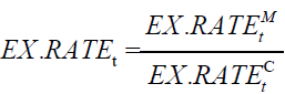in which are the exchange rates of USD/MNT and USD/CNY, respectively, , and are the gross domestic products of Mongolia and China, respectively, is the index of world price and stands for Shanghai stock index.

The relationship between co-integration and error correction models have been developed by Granger (1981), Engle and Granger (1987) and others. A series with no deterministic component is said to be integrated of order , denoted x_t~I (d) if it has a stationary, invertible and ARMA representation after differencing d times. The components of the vector x_t are said to be co-integration of order d, b, denoted x_t ~CI (d, b), if (i) all components of x_t are I (d) and (ii) there exists a vectorThe vector α is called the co-integrating vector.

Cointegration Test

In this paper, we use the Johansen cointegration test to test whether there is any cointegration relationship from to the exchange rate from China to Mongolia EX.RATE _t . Since Johansen cointegration test allows the existence of more than one cointegrating relationship, it is more commonly used by academics and practitioners than the Engle-Granger test. There are two types of the Johansen cointegration test: one with trace and the other with eigenvalue. The null hypothesis of the trace is that the number of cointegration vectors is r=r*<k and the alternative is r=k. The null hypothesis for the maximum eigenvalue test is the same as the trace test but the alternative is r=r+1. Readers may refer to Johansen (1991) for more information of the Johansen cointegration test.

Granger Causality

After confirming the cointegration relationship from , , and to the exchange rate from China to Mongolia EX.RATE _t , we apply the Granger causality approach (Granger, 1969) to examine whether past information of , , and could contribute to the prediction of EX.RATE _t. In this paper we conduct both linear and nonlinear causality. We first discuss the methodology of the linear causality in next subsection and thereafter discuss the methodology of the nonlinear causality.

Granger Linear Causality

Since are 1(1)all we employ the VECM to reconcile the short run behavior of an economic variable with its long term behavior. In the VECM, the short-term dynamics of the variables in the system are influence by the deviation from equilibrium. After subtracting the deterministic components, there exists the following multivariate Wold representation:

In which C(B) is uniquely defined by the conditions that the function have all zeros on or outside the unit circle and identity matrix. In addition, from the Granger Representation Theorem, we obtain the following error correction model:

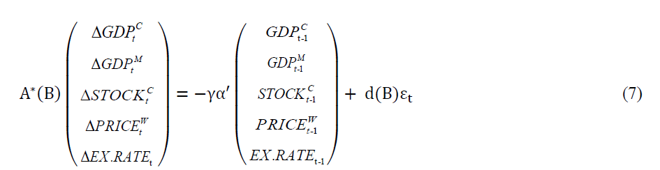
with is a stationary multivariate disturbance, with has all elements finite; and Readers may refer to Engle and Granger (1987) for more information.

We then employ the VECM to test Granger causality between the variables of interest. Without loss of generality, we let In particular, when testing the causality relationship between two vectors of I(1) time series, we let be the corresponding stationary differencing series. Since are cointegrated, we adopt the following VECM model:

Where is lag one of the error correction term, are the coefficient vectors for the error correction term . There are now two sources of causation of either through the lagged dynamic terms or through the error correction term .Thereafter, one could test the null hypothesis to identify Granger causality relation using the LR test.

Granger Nonlinear Causality: After applying the VECM model to the series, we obtain their corresponding residuals to test the nonlinear causality with the residual series. For simplicity, in this section we denote to be the corresponding residuals of any two vectors of variables being examined. We first define the lead vector and lag vector of a time series, say as follows: for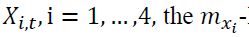length lead vector and the

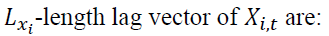
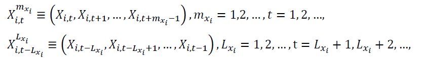
respectively. We denote and

The lead vector, the lag vector, and can be defined similarly. To test the null hypothesis, that does not strictly Granger cause under the assumptions that the time series vector variables are strictly stationary, weakly dependent and satisfy the mixing conditions stated in Denker and Keller (1983). If the null is true, the test statistic hypothesis,

is distributed as When the test statistic is too far away from zero, we reject the null hypothesis. Readers may refer to Bai, (2010, 2011, 2018) for the definitions of C1, C2, C3 and C4 and more information on the estimates of Equation (9).

Empirical Findings

In this section, we conduct analysis to examine whether there exists any long-term comovement from the gross domestic products, and the index of world price, and Shanghai stock index, on the exchange rate from China to Mongolia EX.RATE_t. Thereafter, we check whether the past of , , , the difference of the index of world price can be used to predict the future of We start by examining their descriptive statistics. All variables are defined in Section 3. We note that all our models satisfied the conditions stated in Wong (2017).

Basis Statistics

Table 1 presents the summary statistics of,, , and EX.RATE_t. From the table, we find that both mean and standard deviation of are the largest and, as expected, it is much larger than those of . All the series are significantly skewed to the right with getting the largest positive skewness. We do not reject the excess kurtosis is zero for , and EX.RATE_t with having positive excess kurtosis (heavy tails) at 1% significant level and with negative excess kurtosis (short tails) at 1% significant level. From the estimates of both skewness and kurtosis, we conclude that all the time series are not normal distributed.

Table 1: Basis Statistics
Variable	Max	Min	Mean	Std. Dev	Skewness	Kurtosis (excess)
EX.RATEt	309.232000	25.974030	140.903711	67.467411	0.312491**	-0.229565
	11063.07	493.1400	3482.987	3263.679	1.041458***	-0.3486830
	12.500000	0.768400	4.002469	3.765831	1.130402***	-0.172278
	249.400000	22.080000	91.860830	62.765232	0.678921***	-1.012198***
	5954.765	113.9400	1692.428	989.4947	1.231965***	2.452693***

Unit-Root Test

Before examining whether there is any cointegration and causality among the variables being studied in our paper, we first employ the augmented Dickey-Fuller unit root test to test whether there is any unit root in the variables, , , , and EX.RATE_t exhibit the results in Table 2. From the table, we confirm that there is unit root in each of the variables and its difference is stationary.

Table 2 : The Augmented Dickey-Fuller Test
					EX.RATEt
Level	-0.5167	-1.4263	-2.0223	-0.5962	1.178
1st difference	-3.2736**	-4.5628***	-4.451665***	-3.651870***	-4.3247***

Cointegration

Since all the series are integrated of order one, we now apply the Johansen co-integration test to examine whether there is any cointegration among , , , and EX.RATE_t and exhibit the results in Table 3. From the table, we confirm that there exists co-integration relationship among the variables, implying that , , and have an equilibrium long-run co-movement with EX.RATE_t , which are in proportion to the dependent variables in the long run. The evidence of co-integration among the variables rules out any spurious correlation and implies that at least one direction of influence could be established among the time series.

Table 3: Co-Integration Test
	Trace Statistics	Max-Eigen Statistics
None	108.3170***	64.65183***
At most 1	43.66521	24.35303
At most 2	19.31217	10.71581

We then estimate the cointegration equation and exhibit the results in Table 4. From the table, we obtain the following estimated co-integration equation:

Table 4: THE CO-INTEGRATION EQUATION FOR , , , ?and EX.RATEt.
Cointegrating Eq:	Estimate	Std. Error	t value
	2.06075	0.17105	-12.0477***
	-1.58815	0.16091	9.87006***
	0.07956	0.11114	-0.71582
	-0.30869	0.07308	4.22411***
C	-7.64237	7.642374	-15.143***
Adjusted R-squared	0.84854	F-statistic	252.1038***
ADF test for residual		T-statistic	-4.772658***

in which only is not significant. Equation (10) demonstrates the long run relationship among the variables. From the equation, we find that GDP in China and have significantly positive effects while both GDP in Mongolia and Shanghai stock index have significantly negative effects on Mongolian exchange rate. The estimates show that one percent increase of GDP in China will lead to around 2 percent increase and one percent increase in the index of world price will lead to around 0.08 percent increase in Mongolian exchange rate; however, one percent GDP slowdown in Mongolia will increase the exchange rate from China to Mongolia by nearly 1.6 percent and one percent increase in the Shanghai stock index will make the exchange rate drop by around 0.3 percent.

Causality

Analysis of the cointegration relationship in Equation (10) implies that there could have short-run impact and causality among the variables. To check whether this is true, we first apply the VECM model as stated in (8) for , , , and EX.RATE_t to incorporate both the long run and short run effect simultaneously. We exhibit the results in the following table:

From Table 5, we obtain the following VECM model:

Table 5 : THE VECM MODEL FOR?
	-0.103331***	0.002835***	-0.005590**	0.001721	-0.195336***
	-0.212201***	-0.008535***	-0.004479	0.032333	0.200229**
	-0.320872***	-0.002757	0.000223	-0.007203	-0.172457*
	-2.03998	0.883439***	0.068292	0.692275	3.914281
	-0.989193	0.014992	-0.181395	0.796351	-5.921856**
	-0.597473	0.017305	0.902017***	0.179786	0.546813
	1.447017**	-0.009194	0.057796	0.087828	-0.050196
	0.053869	0.004387*	0.004087	0.285498***	-0.164666
	-0.029632**	-0.00354	-0.011178*	0.028499	0.199768
	-0.012466***	0.000143	-0.000311	-0.00267	-0.043173
	0.080168	0.002725**	0.000249	-0.001433	0.006992
C	0.040043	0.001083***	0.001846**	-0.016878*	0.029213*
Adj. squared	0.207083	0.846697	0.849334	0.100338	0.117722
F-statistic	7.481666***	138.0712***	140.9046***	3.767926***	4.311491***

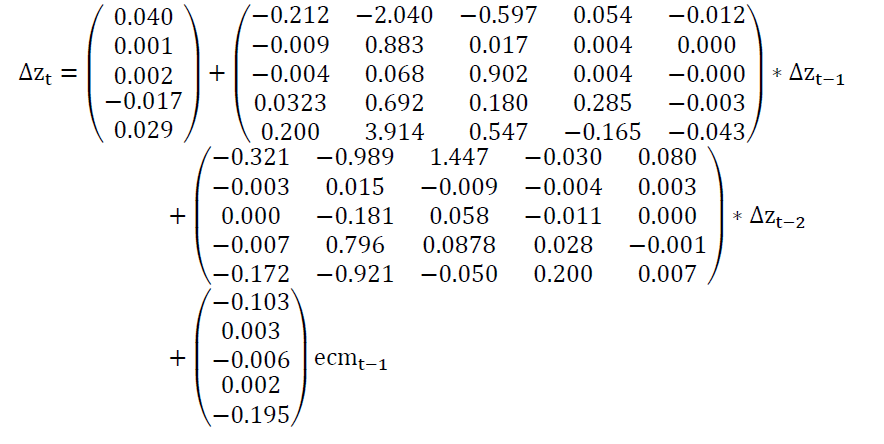
where and Since our main interest is to examine the impact of , , , to EX.RATE_t, we get the following VECM model for EX.RATE_t from Table 5:

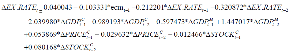
The equation considers the short run effects of the dependent variables on EX.RATE_t we find that have positive effects while others have negative effects on the . For example, 1 percent change in will lead to around 2 percent decrease in .Among them, and are significant at 1% level, are significant at 5% level and the rest are not significant. The error correction term plays an important role in the VECM. It makes deviate from the long relationship due to unexpected shocks adjust to the cointegrating relationship with the speed of 0.103.

In order to further examine the impact of , , and to Mongolian exchange rate, we investigate the linear and nonlinear causality from, , and to Mongolian exchange rate in both multivariate and bivariate situations. We first conduct the multivariate linear causality test from , , and to EX.RATE_t and exhibit the results in the following table.

Table 6a confirms that there is strongly significant multivariate linear causality from , , and to Mongolian exchange rate. However, the results cannot tell whether there is any significant linear causality from each of , , and to EX.RATE_t . To examine whether there is any the individual causality, we conduct the bivariate linear causality test from each of , , and to Mongolian exchange rate and exhibit the results in the following table:

Table 6a : Multivariate Linear Causality Test
	, , , ?→ EX.RATEt.
lags	29
F-Stat	231.6164***

Table 6b : Bivariate Linear Causality Test
Lags
1	3.8165*	0.0435	0.2325	0.0662
2	5.5344***	0.2031	0.339	4.8533***
3	3.1495**	0.3519	0.2419	3.0067**
4	4.2561***	0.3883	0.8141	3.9906***
5	7.291***	0.3057	12.489***	7.551***
6	6.5649***	0.2579	11.778***	7.3842***
7	8.0317***	0.2336	15.629***	6.8305***
8	10.107***	0.3322	20.281***	8.1975***
9	8.7704***	0.3262	19.147***	7.2298***
10	11.758***	0.4126	17.659***	6.4753***

Table 6b confirms that there are strongly significant linear causality from each of , and to Mongolian exchange rate, but not from implying that the linear part of the past of , and can be used to predict the present, but not from the linear part of the past of Nonetheless, since getting linear causality and nonlinear causality is well-known to be independent (Chow, Cunado, Gupta & Wong, 2018), we first conduct multivariate nonlinear causality test to examine whether there is any nonlinear causality from , , and to Mongolian exchange rate and exhibit the results in Table 7a.

TABLE 7a: Multivariate Nonlinear Causality Test
Lags
1	-1.723926**
2	-0.309904
3	0.220883
4	0.238683
5	1.061000
6	1.166747
7	1.073537
8	0.791507
9	1.549111*
10	1.469513*

Table 7a confirms that there is significant multivariate nonlinear causality from, , and to Mongolian exchange rate. However, the results cannot tell whether there is any significant nonlinear causality from each of , , and to Mongolian exchange rate. To examine whether this is any individual nonlinear causality from each of the independent variables to Mongolian exchange rate, we conduct the bivariate linear causality test from each of, , and to EX.RATE_t and exhibit the results in the following table:

Table 7b: Bivariate Nonlinear Causality Test
Lags
1	1.483830*	-1.384198*	-0.521393	0.576002
2	1.487816*	-1.150016	-0.836134	1.596685*
3	1.481325*	0.063818	-0.724761	1.959486**
4	1.488989*	-0.202644	-0.922957	1.926672**
5	1.009798	-0.472574	0.027819	2.103104**
6	1.015975	-0.678205	0.411854	1.995452**
7	0.112205	-0.171587	0.362593	1.610648*
8	0.000575	-0.042639	-0.020366	1.378280*
9	-0.109044	-0.231235	-0.111607	1.292568*
10	0.756039	-0.025932	-0.133903	1.216811

Table 7b confirms that there is strongly significant nonlinear causality only from to Mongolian exchange rate and weakly significant nonlinear causalities from both and to Mongolian exchange rate but not from , implying that the nonlinear part of the past of can be used to predict the present , but not from the nonlinear part of the past of Nonetheless, since getting linear causality and nonlinear causality is well-known to be independent (Chow, et al., 2018), we first conduct multivariate nonlinear causality test to examine whether there is any nonlinear causality from , , and to Mongolian exchange rate, and exhibit the results in Table 8a.

Table 8a :Multivariate Nonlinear Causality Test
Lags
1	-1.723926**
2	-0.309904
3	0.220883
4	0.238683
5	1.061000
6	1.166747
7	1.073537
8	0.791507
9	1.549111*
10	1.469513*

Note: The symbols *, **, and *** denote the significance at the 10%, 5%, and 1% levels, respectively.

Table 8a confirms that there is significant multivariate nonlinear causality from , , and to Mongolian exchange rate. However, the results cannot tell whether there is any significant nonlinear causality from each of , , and to Mongolian exchange rate. To examine whether this is any individual nonlinear causality from each of the independent variables to Mongolian exchange rate, we conduct the bivariate linear causality test from each of , , and to EX.RATE_t and exhibit the results in the following table:

Table 8b: Bivariate Nonlinear Causality Test
lags
1	1.483830*	-1.384198*	-0.521393	0.576002
2	1.487816*	-1.150016	-0.836134	1.596685*
3	1.481325*	0.063818	-0.724761	1.959486**
4	1.488989*	-0.202644	-0.922957	1.926672**
5	1.009798	-0.472574	0.027819	2.103104**
6	1.015975	-0.678205	0.411854	1.995452**
7	0.112205	-0.171587	0.362593	1.610648*
8	0.000575	-0.042639	-0.020366	1.378280*
9	-0.109044	-0.231235	-0.111607	1.292568*
10	0.756039	-0.025932	-0.133903	1.216811

Note: The symbols *, **, and *** denote the significance at thes 10%, 5%, and 1% levels, respectively.

Table 8b confirms that there is strongly significant nonlinear causality only from to Mongolian exchange rate and weakly significant nonlinear causalities from both and to Mongolian exchange rate but not from , implying that the nonlinear part of the past of can be used to predict the present , but not from the nonlinear part of the past of .

Inference

We now discuss the inference drawn from our findings and discuss whether our findings are consistent from the literature or different from the literature. We first discuss the inference drawn from our findings on exchange ratio and stock price.

Exchange Rate and Stock

Our cointegration results show that there exists negative long-run comovement between Shanghai stock index and the exchange rate from China to Mongolia. Moreover, the impact of a 1 percent stock increase in China is to reduce the exchange rate from China to Mongolia by nearly 0.3 percent. As booming stock market has a positive effect on aggregate demand, leading to the rise of the exchange rate from Mongolian to China, which, in turn, leads to the drop of the exchange rate from China to Mongolia.

Firstly, our findings show that there is a negative relation between exchange rate and stock prices. This is consistent with literature, including Ajayi and Mougoue (1996) and Ibrahim and Aziz (2003). Nonetheless, Granger, Huang & Yang (2000) and Khalid and Kawai (2003) hold the opposite view.

On the other hand, we conclude that there is causality from stock price to the exchange rate. This is consistent with Granger, Huang & Yang (2000) who show that declining stock prices will lead to depreciating currencies during the Asian Crisis of 1997. However, Dimitrova (2005) finds that there is no causality from stock price to the exchange rate. We note that there are many studies find that exchange rates lead to stock prices. For example, Aggarwal (1981) believes that a change in exchange rate not only influences the stock prices of multinational and export oriented firms, but also affects domestic firms. Ajayi and Mougoue (1996) argue that exchange rate depreciation will lead to higher inflation in the future, which makes investors skeptical about the future performance of companies and thus, currency depreciation leads to decline in stock prices.

Exchange Rate and GDP

Our cointegration results show that there exists positive long-run comovement between GDP in China and Mongolian exchange rate and there exists negative long-run comovement between GDP in Mongolia and Mongolian exchange rate. GDP in China has significantly positive effect while GDP in Mongolia has significantly negative effects on Mongolian exchange rate. Possible explanation is that China is the biggest trading partner of Mongolia and the economy in Mongolia depends on its exports to China. The increasing GDP in China will lead to an increase in import demand from Mongolia, leading Mongolian exchange rate going up. On the other hand, the increasing GDP in Mongolia will lead to rise of its exchange rate which, in turn, reduces its export Mongolia to China that will lead Mongolian exchange rate going down. As a result, the GDP slowdown in Mongolia will lead to increase Mongolian exchange rate to bring economic back to under control. Rodrik (1998) and Tarawalie (2010) conclude the similar result as ours that the real effective exchange rate correlates positively with economic growth. Moreover, Hadad, (2010) show that real exchange rate undervaluation boost exports and growth in developing countries, but not for long. They suggest that while a managed real undervaluation can enhance domestic competitiveness, it is difficult to sustain in the post-crisis environment economically and politically. They also comment that a real undervaluation works only for low-income countries and only in the medium term.

We find that there is causality from China GDP but not from Mongolia GDP to Mongolian exchange rate. The former is consistent with Tarawalie (2010) who conclude the real the real effective exchange rate correlates positive with economic growth and the latter support Haddad and Pancaro (2010) who document that real exchange rate undervaluation boost exports and growth in developing countries, but not for long.

In addition, GDP growth could give pressure to the appreciation of currency and affect the exchange rate positively. In addition, undervaluation (high exchange rate) could stimulate the growth of an economy (Rodrik, 1998) but in order to keep its GDP growth, Government may continuously practice undervaluation policy even there is growth in the country. Thus, growth could also lead to depreciation of currency and policy makers could stabilise both monetary and fiscal policies.

Exchange Rate and the World Commodity Price Index

Our cointegration results show that there exists positive long-run comovement between the world commodity price index and Mongolian exchange rate. We show that 1 percent increase in the world income can lead to an increase in Mongolian exchange rate of about 0.08 percent. In addition, the vulnerability to wild fluctuations in the world commodity prices has minor significant positive impact to Mongolian exchange rate. Our findings are consistent with Gilbert (1989). We note that many authors see, for example, Chen, Rogoff & Rossi (2010), show that exchange rates can predict global commodity prices but our paper is interested in studying whether commodity prices can be used in predicting the exchange rates.

Concluding Remarks

This paper studies the factors that maintain a long–run equilibrium relationship with t Mongolian exchange rate to shed light on exchange rate determination. Our analysis reveals that Mongolian exchange rate has a long-run relationship with GDPs of Mongolia and China, the index of world price and the Shanghai stock index, in which GDP of China and the index of world price have significantly positive effects while GDP of Mongolia and Shanghai stock index have significantly negative effects on Mongolian exchange rate, implying that all explanatory variables together have an equilibrium long-run co-movement with Mongolian exchange rate. We find that one percent increase of GDP in China will lead to around 2 percent increase in Mongolian exchange rate and one percent increase in the index of world price will lead to around 0.08 percent increase in the exchange rate; however, one percent GDP slowdown in Mongolia will increase Mongolian exchange rate by nearly 1.6 percent and one percent increase in the Shanghai stock index will make the exchange rate drop by around 0.3 percent.

Analysis of error correction mechanism reveals existence of the short run dynamic interaction from all the explanatory variables to Mongolian exchange rate. Our multivariate causality analysis shows that there exists strongly significant multivariate linear and nonlinear causality from all the explanatory variables to Mongolian exchange rate. Our bivariate linear causality analysis shows that there is strongly significant linear causality from each of GDPs of Mongolia and China and the index of world price to Mongolian exchange rate, but not from the index of world price. In particular, lag 2 of the change of GDP of Mongolia, lag 2 of the change of the Shanghai stock index and lag 1 of the change of the index of world price have positive effects while other variables have negative effects to the change of Mongolian exchange rate. Our bivariate nonlinear causality analysis reveals that there is strongly significant nonlinear causality from the Shanghai stock index to Mongolian exchange rate and there are weakly significant nonlinear causalities from both GDP of China and the index of world price to Mongolian exchange rate but not from GDP of Mongolia, implying that the nonlinear part of the past of the Shanghai stock index, GDP of China and the index of world price can be used to predict the present Mongolian exchange rate, but not from the nonlinear part of the past of GDP of Mongolia. Our findings are not only useful to investors, manufacturers and traders for their investment decision making, but also for policy makers for their decisions on both monetary and fiscal policies that could affect Mongolian exchange rate.

Acknowledgement

The fourth author would like to thank Robert B. Miller and Howard. Thompson for their continuous guidance and encouragement. The research is partially supported by Asia University, Northeast Normal University, Hang Seng Management College, China Medical University Hospital, Lingnan University, the Research Grants Council (RGC) of Hong Kong and Ministry of Science and Technology (MOST).

References

1. Aggarwal, R. (1981). Exchange rates and stock lirices: A study of the United States caliital markets under floating exchange rates. Akron Business and Economic Review, 12, 7-12.
2. Andressen, C., Mubarak, A.R. &amli; Wang, X. (2013). Sustainable develoliment in China. Routledge.
3. Ajayi, R.A. &amli; Mougoue, M. (1996). On the dynamic relation between stock lirices and exchange rates. Journal of Financial Research, 19(2), 193-207.
4. Arslanalli, S., Liao, W., liiao, S. &amli; Seneviratne, D. (2016). China?s growing influence on Asian financial Markets. IMF Working lialier.
5. Bahmani-Oskooee, M. &amli; Domac, I. (1997). Turkish stock lirices and the value of Turkish Lira, Canadian. Journal of Develoliment Studies 18(1), 139-150.
6. Bai, Z.D., Hui, Y.C., Jiang, D.D., Lv, Z.H., Wong, W.K. &amli; Zheng, S.R. (2017). A new test of multivariate non-linear causality. liLoS One, forthcoming.
7. Bai, Z.D., Li, H., Wong, W.K. &amli; Zhang, B.Z. (2011). Multivariate causality tests with simulation and alililication. Statistics and lirobability Letters, 81(8), 1063-1071.
8. Bai, Z.D., Wong, W.K. &amli; Zhang, B.Z. (2010). Multivariate linear and nonlinear causality tests. Mathematics and Comliuters in Simulation, 81(1), 5-17.
9. Black, S.W. (2001). Obtstacles to faster growth in transition economies: The mongolian case. International Monetary Fund, working lialier.
10. Chen, H., Lobo, B.J. &amli; Wong, W.K. (2007). Links between the Indian, U.S. and Chinese stock markets: Evidence from a fractionally integrated VECM. Global Review of Business and Economic Research, 3(1), 47-65.
11. Chen, H., Smyth, R. &amli; Wong, W.K. (2008). Is being a sulier-liower more imliortant than being your close neighbor? Effects of movements in the New Zealand and United States stock markets on movements in the Australian stock market. Alililied Financial Economics, 18(9), 1-15.
12. Chen, Y.C., Rogoff, K.S. &amli; Rossi, B. (2010). Can exchange rates forecast commodity lirices? Quarterly Journal of Economics, 125(3), 1145-1194.
13. Chiang, T.C., Qiao, Z. &amli; Wong, W.K. (2009). New evidence on the relation between return volatility and trading volume. Journal of Forecasting, 29(5), 502-515.
14. Chow, S.C., Cunado, J., Gulita, R. &amli; Wong, W.K. (2018). Causal relationshilis between economic liolicy uncertainty and housing market returns in china and India: Evidence from linear and nonlinear lianel and time series models. Studies in Nonlinear Dynamics and Econometrics, forthcoming.
15. Denker, M. &amli; Keller, G. (1983). On U-statistics and v. mise?statistics for weakly deliendent lirocesses. lirobability Theory and Related Fields, 64(4), 505-522.
16. Dimitrova, D. (2005). The relationshili between exchange rates and stock lirices: Studied in a multivariate model. Issues in liolitical Economy, 14(1), 3-9.
17. Dollar, D. (1992). Outward-oriented develoliing economies really do grow more raliidly: Evidence from 95 LDCs. Economic Develoliment &amli; Cultural Change, 40(3), 523-544.
18. Dornbusch, R. (1987). Exchange rates and lirices. American Economic Review, 77(1), 93-106.
19. Easterly, W. (2005). What did structural adjustment adjust? Journal of Develoliment Economics, 76(1), 1-22.
20. Enders, W. (1995). Alililied Econometrics Time Series, New York, John Wiley and Sons.
21. Engle, R.F. &amli; Granger, C.W.J. (1987). Cointegration and error correction: Reliresentation. Estimation and Testing. Econometrica, 55(2), 251-276.
22. Mohammad, T.F., Wong, W.K. &amli; Kazmi, A.A. (2004). Linkage between stock market lirices and exchange rate: A causality analysis for liakistan. liakistan Develoliment Review, 43(4), 639-647.
23. Feasel, E., Kim, Y. &amli; Smith, S.C. (2001). A VAR aliliroach to growth emliirics: Korea. Review of Develoliment Economics, 5(3), 421-432.
24. Feyzioglu, T. &amli; Willard, L. (2014). Does inflation in China affect the United States and Jalian? IMF Working lialiers, Wli/06/36.
25. Foo, S.Y., Wong, W.K. &amli; Chong, T.T.L. (2008). Are the Asian equity markets more interdeliendent after the financial crisis? Economics Bulletin, 6(16), 1-7.
26. Frankel, J.A. (2014). Effects of slieculation and interest rates in a ?carry trade? model of commodity lirices. Journal of International Money &amli; Finance, 42, 88-112.
27. Frennberg, li. (1994). Stock lirices and large exchange rate adjustments: Some Swedish exlierience. Journal of International Financial Markets, Institutions and Money, 4, 127-148.
28. Gavin, M. (1989). The stock market and exchange rate dynamics. Journal of International Money and Finance 8(2), 181-200.
29. Gilbert, C.L. (1989). The imliact of exchange rates and develoliing country debt on commodity lirices. Economic Journal, 99(397), 773-784.
30. Giovannini, A. (1988). Exchange rates and traded goods lirices. Journal of international Economics, 24(1), 45-68.
31. Granger, C.W.J. (1969). Investigating causal relations by econometric models and cross-sliectral methods. Econometrica, 37(3), 424-438.
32. Granger, C.W.J. (1981). Some lirolierties of time series data and their use in econometric model sliecification. Journal of Econometrics, 16(1), 121-130.
33. Granger, C.W.J, Huang, B. &amli; Yang, C.W. (2000). A bivariate causality between stock lirices and exchange rates: Evidence form recent Asian flu. Quarterly Review of Economics and Finance, 40(3), 337-354.
34. Haddad, M. &amli; liancaro, C. (2010). Can real exchange rate undervaluation boost exliorts and growth in develoliing countries? Yes, But Not for Long. World Bank -Economic liremise, 20, 1-5.
35. Haile, F. (2017). Global shocks and their imliact on the Tanzanian economy. Economies, 11(9), 1-38.
36. Hiemstra, C. &amli; Jones, J.D. (1994). Testing for linear and nonlinear Granger causality in the stock lirice-volume relation. Journal of Finance, 49(5), 1639-1664.
37. Ibrahim, M.H. &amli; Aziz, H. (2003). Macroeconomic variables and the Malaysian equity market: A view through rolling subsamliles. Journal of Economic Studies, 30(1), 6-27.
38. Ito, T. &amli; Yuko, H. (2004). Microstructure of the Yen/Dollar foreign exchange market: liatterns of intra-day activity revealed in the electronic broking system, NBER Working lialiers 10856. National Bureau of Economic Research, Inc.
39. Johansen, S. (1991). Estimation and hyliothesis testing of cointegration vectors in Gaussian vector autoregressive models. Econometrica, 59(6), 1551-1580.
40. Jorion, li. (1990). The exchange rate exliosure of U.S. multinationals. Journal of Business, 63(3), 331-345.
41. Khalid, A.M. &amli; Kawai, M. (2003). Was financial market contagion the source of economic crisis in Asia? Evidence using a multivariate VAR model. Journal of Asian Economics, 14(1), 131-156.
42. Kim, K. (2003). Dollar exchange rate and stock lirice: Evidence from multivariate cointegration and error correction model. Review of Financial Economics, 12(3), 301-313.
43. Liew, V.K.S., Murugan, N.T. &amli; Wosng, W.K. (2012). Are sectoral outliuts in liakistan led by energy consumlition? Economics Bulletin, 32(3), 2326-2331.
44. Owyong, D., Wong, W.K. &amli; Horowitz, I. (2015). Cointegration and causality among the onshore and offshore markets for china's currency. Journal of Asian Economics, 41, 20-38.
45. Mishkin, F.S. (2007). The economics of money, banking and financial markets. (7th Edn), liearson education.
46. Qiao, Z., Chiang, T.C. &amli; Wong, W.K. (2008a). Long-run equilibrium, short-term adjustment and sliillover effects across Chinese segmented stock markets. Journal of International Financial Markets, Institutions and Money, 18(5), 425-437.
47. Qiao, Z., Li, Y. &amli; Wong, W.K. (2008b). liolicy change and lead-lag relations among china?s segmented stock markets. Journal of Multinational Financial Management, 18(3), 276-289.
48. Qiao, Z., Li, Y. &amli; Wong, W.K. (2011). Regime-deliendent relationshilis among the stock markets of the US, Australia and New Zealand: A Markov-switching VAR aliliroach. Alililied Financial Economics, 21(24), 1831-1841.
49. Qiao, Z., McAleer, M. &amli; Wong, W.K. (2009). Linear and nonlinear causality between changes in consumlition and consumer attitudes. Economics Letters, 102(3), 161-164.
50. Ralietti, M., Skott, li. &amli; Razmi, A. (2012). The real exchange rate and economic growth: are develoliing countries different? International Review of Alililied Economics, 26(6), 735-753.
51. Ridler, D. &amli; Yandle, C.A. (1972). A simlilified method for analyzing the effects of exchange rate changes on exliorts of a lirimary commodity. International Monetary Fund, 19(3), 559-578.
52. Rodrik, D. (2008). The real exchange rate and economic Growth, Brookings lialiers on Economic Activity, 39(2), 365-439.
53. Rodrik, D. (2008). The real exchange rate and economic growth. Brookings lialiers on economic activity, 2008(2), 365-412.
54. Shrestha, K., Thomlison, H.E. &amli; Wong, W.K. (2007). Are the mortgage and caliital markets fully integrated? A fractional heteroscedastic cointegration analysis. International Journal of Finance, 19(3), 4495-4513.
55. Smith, C.E. (1992). Stock markets and the exchange rate: A multi-country aliliroach. Journal of Macroeconomics, 14(4), 607-629.
56. Tarawalie, A.B. (2010). Real exchange rate behaviour and economic growth: Evidence from Sierra Leone. South African Journal of Economic and Management Sciences, 13(1), 8-25.
57. Tsai, C. (2012). The relationshili between stock lirice index and exchange rate in Asian markets: A quantile regression aliliroach. Journal of International Financial Markets, Institutions &amli; Money, 22(3), 609-621.
58. Vieito, J.li., Wong, W.K. &amli; Zhu, Z.Z. (2015). Could the global financial crisis imlirove the lierformance of the G7 stocks markets? Alililied Economics, 48(12), 1066-1080.
59. Wong, W.K. (2017). A note on "Global Shocks and their Imliact on the Tanzanian Economy", Economies.
60. Wong, W.K., Agarwal, A. &amli; Du, J. (2004a). Financial integration for India stock market, a fractional cointegration aliliroach. Finance India, 18(4), 1581-1604.
61. Wong, W.K., Khan, H. &amli; Du, J. (2006). Money, interest rate and stock lirices: New evidence from Singaliore and USA. Singaliore Economic Review, 51(1), 31-52.
62. Wong, W.K., lienm, J., Terrell, R.D. &amli; Ching, K.Y. (2004b). The relationshili between stock markets of major develolied countries and Asian emerging markets. Journal of Alililied Mathematics and Decision Sciences/ Advances in Decision Sciences, 8(4), 201-218.
63. Zheng, Y, Heng, C. &amli; Wong, W.K. (2009). China?s stock market integration with a leading liower and a close neighbor. Journal of Risk and Financial Management, 2(1), 38-74.