keywords

Bank NIM, Oligopoly Market, Game Theory, Ho and Saunders Model.

JEL

G21, C7, L1

Introduction

As an intermediary institution, banks play several important roles in the economy. Banks accept deposits from parties with excess funds and distribute them to those that need funds, namely households, large companies, small- and medium-sized firms, and the government (Berger et al., 2020). The process for receiving deposits and channeling loans takes place in the form of interest charges for savers and borrowers. Under ideal conditions, banks pay lower interest rates to depositors and charge higher interest rates to borrowers. In this case, the net interest margin is the difference between the interest earned and the interest charged by the bank divided by the total productive assets (Tarus et al., 2012).

A bank's NIM is a reflection of two banks’ performance at the same time as a measure of the profits of the bank (Chen & Liao, 2011) and as an illustration of the level of bank efficiency (Drakos, 2003; Beck & Hesse, 2009; Lopes-Espinosa et al., 2011; Sidabalok & Viverita, 2011; Trinugroho et al., 2014). The higher the bank's NIM, the higher the bank's profit. On the other hand, high bank NIM represents an inefficient banking system (Saksonova, 2014).

Its market structure influences the level of efficiency of the banking system. The market structure will influence bank performance, including bank profit level (Wu et al., 2018; Mirzaei et al., 2013; Berger, 1995). In the uncompetitive banking market structure, banks have the power to control prices. Banks will provide lower deposit rates and charge higher loan interest rates. Thus, in an uncompetitive market structure, the bank will produce a higher NIM than the competitive market (Berger, 1995). In contrast, in the competitive banking market structure, the market will encourage banks to set a low NIM (Sensarma & Ghosh, 2004).

There are currently more uncompetitive banking market structures in developing and developed countries (Kasman, 2010). Most developing countries have uncompetitive market structures, as reflected by high NIM (Goddard et al., 2011), such as in Uganda (Beck & Hesse, 2009), Pakistan (Khawaja & Din, 2007), Mexico (Maudos & Solis, 2009), and Indonesia (Sidabalok & Viverita, 2011; Rosengard & Prasetyantoko, 2011; Trinugroho et al., 2014).

Some developed countries also have an uncompetitive market structure. For example, Kasman (2010) finds that most European Union (EU) countries have an uncompetitive banking system. The system includes a monopolistic, collusive oligopoly, and competitive banking system.

Many countries still have an uncompetitive banking market structure, so the model used is a model that fits this market structure (Beck et al., 2004). Several markets are contained in an uncompetitive market structure, namely monopoly, oligopoly, and monopolistic competition (Mankiw, 2015). However, the type of uncompetitive market by the banking market structure is an oligopoly market that only consists of a few banks (Freixas & Rochet, 2008).

Companies are usually divided into two main groups in an oligopoly market: companies with large assets and small assets. Large companies are usually the leaders who decide and make the first decisions, while small companies are usually followers who make decisions following large companies' decisions (Gibbon, 1992). This condition occurs because the large company usually has a lower cost function than the small company to operate more efficiently (Huck, Konrad & Muller, 2001).

1. So far, the model to determine the bank's NIM that bank researchers and practitioners commonly use is the NIM model for competitive markets, namely the Risk Averse Dealer model developed by Ho & Saunders (1981). The Risk Averse Dealer Model is a model used to determine the determinants of a bank's NIM. The Risk Averse Dealer Model can also determine the optimal NIM before the bank carries out the mark-up (Ho & Saunders, 1981)

The Risk Averse Dealer Model becomes the leading model in the analysis of the determinant banks' NIM theoretically and empirically. The Risk Averse Dealer Model is a combined hedging analysis model (Michaelsen & Goshay, 1967) and the microeconomic model (Pyle, 1972). This model underwent many developments, such as McShane & Sharpe (1985); Allen (1988); Angbazo (1997); Saunders & Schumacher (2000); Entrop et al., (2015).

McShane & Sharpe (1985) add the financial markets interest rate risk to the Ho and Saunders model, which only assumes that banks only face the risk of credit and deposit interest rates. In addition to the Risk-Averse Dealer Model, McShane & Sharpe also included time assumptions. In developing the model, McShane & Sharpe (1985) assume that, at the beginning of the period, the bank will set interest rates on deposits and credits based on the risk-free rate in financial markets. McShane & Sharpe assume that, during the period between the beginning and the end of loan and deposits, the bank can accept new deposits or credits so that the bank's risks increase. When the amount of deposits earned by the bank is higher than the loan given, they will face the risk of money market interest rate.

In 1981, Allen extended the Ho & Saunders model. Allen (1981) added the assumption that the product owned by the bank is not a single product. The bank may have multi products to obtain profit with the assumption that both products can substitute each other. Furthermore, Angbazo (1997) also tries to develop the Ho & Saunders model. Angbazo (1997) added the risks of default and the interaction between these risks and interest rate risk and incorporated various factors that influence these risks, especially bank-specific factors. Entrop et al., (2015) explored the extent to which interest risk exposure is priced into the bank margin by extending the Ho & Saunders model to capture interest rate risk and expected return from maturity transformation.

Risk Averse Dealer Model assumes that all banks have the same conditions in both the cost and the profit function so that the banks are in perfect competition. The assumptions used by Ho & Saunders are too simple and not following the real condition in the banking industry. However, most of the studies still use the same assumption that all banks are homogeneous. Bank competition conditions are based on cost determination, and the decision is made simultaneously and independently (static decision). These assumptions are suitable for competitive market conditions. Still, there are few NIM determination models in an uncompetitive market with different types of banks, in which business competition is not only based on cost determination. Furthermore, static and dynamic decisions are also made sequentially and interdependently.

Actually, the competition theory development between banks in the uncompetitive market has started since the research conducted by Klein (1971); Monti (1972). This Monti-Klein model is the starting point for developing a model of the bank's profit and cost function in monopoly and oligopoly markets. From this Monti-Klein model, the profit and cost functions for large (leader) and small (follower) banks in the oligopoly market can be obtained (Toolsema & Schoonbeek, 1999). An empirical test of the Monti-Klein model for bank leaders and followers was conducted by Dixit (1986), which focused on competition for loan amounts, deposits, and interest rates. The same research has also been conducted in Indonesia by Abdullah et al., (2016).

To the best of our knowledge, there are limited studies to estimate the optimal banks’ NIM for the oligopoly market, which consists of large and small banks. In contrast, NIM level’s determination is an instrument of competition between banks (Saunders & Schumacer, 2000).

We add some assumptions to the model to make it more suitable for the real conditions. Some of these assumptions are that each bank group has a different cost and profit function, and the decision making in determining NIM is carried out in stages (dynamically).

Thus, this research has two contributions. First, this study extends the Risk Averse Dealer Model for uncompetitive markets. For research simplification, we use the duopoly market structure as part of the oligopoly market structure. The initial Risk Averse Dealer Model will be modified with the Game Theory framework to suit the duopoly market. Game theory is believed to be the most suitable framework for understanding companies' competitive behavior in the duopoly market structure (Church & Ware, 2000). Therefore, to understand the bank's competition in determining its NIM, the Game Theory analytical framework is used.

Second, we provide new empirical findings on the optimal NIM level for large and small banks. So far, it has been difficult to find the optimal NIM using the Risk Averse Dealer model for duopoly market like in developing countries. In the duopoly market, determining the optimal NIM of a bank using the Risk Averse Dealer model is mostly different from the actual NIM because there is an additional interest rate in converting the bank's perception of risk. These additional interests are known as "mark-up" variables and are not directly included in the model. This makes the government and monetary policy authorities found difficulty to assess the existence of optimal NIM.

For the empirical testing, we conducted this research in Indonesia because Indonesia is known to have an uncompetitive banking market structure (Sutardjo et al., 2011; Widyastuti & Armanto, 2013; Adita & Kusuma, 2015; Wibowo, 2017). To develop a Risk Averse Dealer model that is suitable for non-competitive markets, the approach used is Game Theory with an analysis framework of dynamic games of incomplete information (Church & Ware, 2000).

We extend the model by adding the Stackelberg duopoly model. In this model, the small banks' profit function responds to their large's profit function. Based on this function, the small banks make the loan and deposit functions. The large bank also responded equally to the small banks by creating loan and deposit functions adjusted to small banks' loan and deposit functions.

The result shows that the optimal NIM for the small bank's group is always higher than the optimal NIM for the large bank's group. The optimal NIM for small banks group is always smaller than the actual NIM in all bank groups. For all large banks, the optimal NIM is higher than the actual NIM, whereas, for large competitive banks, the optimal NIM of large banks is always lower than the actual NIM. The latter also applies to the uncompetitive large banks.

To check the robustness, we used the One-Sample t-test. We test the difference between the sample mean and its hypothesis value. The test's significance value is always greater than 0.05, which means no difference between the sample mean value and the hypothesis value. Thus, our results are robust. We find that the NIM estimation results using the Game Theory framework are relatively the same and stable in the ten years of observation. The significance value proves that the Risk Averse Dealer Model modified with the Game Theory is more suitable for non-competitive markets.

This paper is organized as follows. Section 2 presents the literature review, in which the paper builds and highlights our contribution. Section 3 describes the research methodology to calculate the optimal NIM using the game theory conceptual framework, and Section 4 presents the extended model of the initial Ho & Saunders model (1981). Section 5 discusses the findings, and Section 6 concludes the paper.

Literature Review

The Ho and Saunders risk-averse dealer model combines the microeconomic theory (Pyle, 1972) and the hedging analysis theory developed by Michaelsen & Goshay (1967). The model developed by Ho and Saunders became the primary model replacing the hedging analysis model previously developed by Michaelsen & Goshay. After that, the Ho and Saunders model and the microeconomic model became a theoretical model widely used in NIM bank research. Subsequent studies developed both of these models but with the addition of assumptions and the addition of variables.

Several studies that develop microeconomic models are researched by Zarruk (1989); Zarruk & Madura (1992); Wong (1997); Wong (2011); Tsai (2013); Niu et al., (2014); Wong (2014). They were researchers who developed and modified Pyle's (1972) initial model.

The risk-averse dealer model has been extended in the theoretical model like a study from McShane & Sharpe (1985); Allen (1988); Angbazo (1997); Entrop et al., (2015). McShane & Sharpe (1985) extended the risk-averse dealer model by adding one assumption to the bank. As Ho & Saunders assumed that banks face only the credit risk and deposit interest rates, McShane & Sharpe (1985) added interest rate risk of financial markets. Additionally, Allen (1988) suggests a model for multi-products, while Angbazo (1997) added institutional factors to the risk variables. Finally, Saunders & Schumacher (2000) added control variables to calculate the actual NIM (pure spread).

Many researchers also carry out empirical tests using the Ho and Saunders model. Sauer & Scheide (1995) used an econometric model (Granger causality test) and found that macroeconomic variables influenced bank decisions in determining NIM. The finding confirmed by Kunt & Huizinga (1999). In addition to macroeconomic variables, Kunt & Huizinga (1999) found that bank-specific and industry-specific influences the determination of NIM. Empirical research was also carried out by Espinosa, Moreno & Gracia (2011); Entrop et al., (2015). They found that macroeconomic variables affect the nature of bank risk aversion, so that macroeconomic variables will affect the NIM level. Furthermore, they found that the bank will calculate various risks and financial conditions, especially conditions of maturity transformation. They argued that the determination of a bank's NIM is significantly affected by its maturity transformation.

Empirical research using the Ho & Saunders model has also been carried out on a country scale, both in developed and developing countries. Some NIM research in developing countries is the study of Beck & Hesse (2008); Maudos & Solis (2009); Khawaja & Din (2007); Wong et al., (2007); Alper & Anbar (2011). In contrast, the NIM research conducted in developed countries included Zhou & Michael (2008), who examined determinant NIM in China and Vilverde & Fernandes (2007); who examined determinant NIM in Europe. However, even though there has been much research on NIM, all the models still use competitive market assumptions.

Islam & Nishiyama (2016) added a few more variables to the Ho and Saunders model. They divided the variables into three main groups: bank-specific, industry-specific, and macroeconomic-specific groups. Nevertheless, there are still very few models that discuss optimal NIM for large banks and small banks in the oligopoly market. Many countries have oligopoly banking market structures, including developed markets, such as the member countries of the European Union (EU) (Kasman, 2010). Therefore, it is interesting to examine optimal NIM for large and small banks in the oligopoly market.

Research Methodology

Data and Methodology

This study uses the annual financial report published by the central bank and Financial Services Authority during the period 2008-2017. We divide the bank's financial statements into two groups. The first group is banks that have assets more than the average bank assets in the industry. The second group is banks that have assets below the average bank assets in the industry. The first group is categorized as large banks that are the leaders in determining the number of loans disbursed, deposits collected, and NIMs. In contrast, a second group is a group of small banks that become followers.

Additionally, to determine NIM, three separate groups are created. The first group is all banks (82 banks, consisting of 68 small banks and 14 large banks). The second group comprises competitive banks with the same power (entering all economic sectors) (30 banks, consists of 24 small banks and six large banks). The third group includes specific banks or uncompetitive banks with special powers in certain markets (62 banks, consisting of 54 small banks and eight large banks).

Variables

The variables consist of two groups: First, to measure the initial Ho and Saunders model. The second group is used for extended Ho and Saunders model the game theory framework. Table 1 presents the variables used to estimate the optimal NIM using the initial model by Ho and Saunders.

Table 1 The Initial Ho And Saunders Model
Variables	Formulas
Net Interest Margin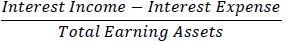
Implicit Interest Expenses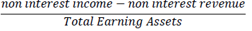
Opportunity Cost of Reserve Requirement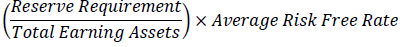
Default Premium of Loans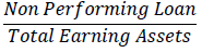

The variables for the extended Ho and Saunders model using the game theory framework (dynamic games of incomplete information) is presented in Table 2 below.

Table 2 The Extended Ho and Saunders Model Using Game Theory Framework
Variables	Formulas
Net Interest Margin*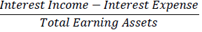
Loans*	Total Loans
Deposits*	(Current Account + Saving Account + Time Deposit)
Interest Rate of Loan*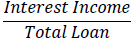
Interest Rate of Deposit*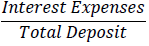
Operational Expenses Other than Interest*	Operational Expenses Other than Interest
Loan Service Fee*	Loan Interest Rate – Risk Free Rate
Deposit Service Fee*	Risk Free Rate – Deposit Interest Rate
Reserve Requirement*	Reserve Requirement
Money Market Position*	Interbank Placement – Interbank Liabilities
Risk Free Rate*	Seven Day Repo Rate
Total Operational Expenses*	Total Operational Expenses
Economic Growth**	GDP Growth
Inflation Rate**	Inflation Rate

Table 3 to Table 5 summarizes the data descriptions for each group, namely all banks, competitive banks and specific banks. In the first group, the number of banks observed was 82 banks. The average NIM of banks in this group was 6.12 percent and fluctuated between -6.25 percent to 17.34 percent. This data indicates that the NIM of banks in this group has a relatively large distribution (the difference in NIM between banks is relatively large).

Table 3 Descriptive Statistics of Research Variables for Groups of 82 Banks Panel Data 2008 – 2017
Variables	Obs	Mean	Std. Dev.	Min	Max
NIM	820	0.0612109	0.0246087	-0.0625	0.1734
Average Loan Interest Rates	820	0.1557795	0.0544118	0.0219355	0.5226414
Average Saving Interest Rates	820	0.0630947	0.0552825	0.003207	0.7906221
Loan Service Fees	820	0.0900295	0.0542985	-0.055565	0.4651414
Saving Service Fees	820	0.0026553	0.05652	-0.725622	0.0801418
Central Bank Interest Rates	820	0.06575	0.014168	0.0425	0.0925
Loans Disbursed (million Rp)	820	28,500,000	79.600.000	34,461	708,000,000
Third-Party Funds (million Rp)	820	33,200,000	95.600.000	27,636	803,000,000
Operational Costs Other than Interest (million Rp)	820	2,125,769	5,540,645	8,022	53,200,000
Fund Position in Money Market (million Rp)	820	760,176	2,313,189	-945,196	17,000,000
Total Operating Costs (million Rp)	820	3,496,877	8,624,820	12,716	81,000,000
Economic Growth	820	0.0551	0.0066764	0.045	0.065
Inflation rate	820	0.05293	0.0239717	0.0275	0.0942

Table 4 presents the statistics of 30 competitive banks. The average NIM in 10 years was 5.38 percent, the highest NIM was 12.37 percent, and the lowest NIM was -6.25 percent. Although the NIM range is high (18.62%), the NIM standard deviation for this group is relatively small, so it can be said that the NIM data is scattered around the average value or the NIM is relatively homogeneous. The average value of credit extended by 30 banks over ten years reached IDR 15.41 trillion, with the largest value reaching IDR 708.01 trillion and the smallest IDR 173.37 billion. The average amount of the Third Party Fund (TPF) collected in 10 years reached IDR 17.38 trillion with the largest IDR 803 trillion values and the smallest value of IDR 177.59 billion. The value of the range - both deposits and credit - is due to the large difference in asset values between large and small banks.

Table 4 Descriptive Statistics of Research Variables For Groups of Competitive Banks Panel Data 2008 – 2017
Variables	Obs	Mean	Std. Dev.	Min	Max
NIM	300	0.053797	0.019008	-0.062500	0.123700
Average Loan Interest Rates	300	0.134959	0.037863	0.031381	0.283363
Average Saving Interest Rates	300	0.059844	0.048842	0.018068	0.790622
Loan Service Fees	300	0.069209	0.038753	-0.043619	0.235863
Saving Service Fees	300	0.005906	0.049690	-0.725622	0.061391
Central Bank Interest Rates	300	0.065750	0.014168	0.042500	0.092500
Loans Disbursed (million Rp)	300	15,412,817.09	7.25	173,374.63	708,010,866.71
Third-Party Funds (million Rp)	300	17,378,771.66	7.43	177,589.50	803,325,062.43
Operational Costs Other than Interest (million Rp)	300	957,451.17	7.73	17,415.00	53,192,076.22
Fund Position in Money Market (million Rp)	300	4,036,344.45	4.53	0.00	28,846,810.78
Total Operating Costs (million Rp)	300	1,972,988.59	6.82	30,868.14	81,017,035.07
Economic Growth	300	0.05510	0.0066924	0.04500	0.06500
Inflation rate	300	0.05293	0.0240293	0.02750	0.09420

Descriptive statistics of specific bank groups can be seen in Table 5. The average NIM for this specific bank is 6.35 percent, and the minimum NIM is 0.0 percent, and the maximum NIM is 17.34 percent. The average loan interest rate for this group is 16.21 percent, with a minimum of 2.19 percent, and the maximum value is 52.26 percent. While the average deposit interest rate reaches 6.35 percent, with the smallest value is 0.32 percent, and the largest value is 74.28 percent.

Table 5 Descriptive Statistics of Research Variables for Groups of Specific Banks Panel Data 2008 – 2017
Variable	Obs	Mean	Std. Dev.	Min	Max
NIM	620	0.0634686	0.0254159	0	0.1734
Average Loan Interest Rates	620	0.1620694	0.0568804	0.021936	0.5226414
Average Saving Interest Rates	620	0.063471	0.0552674	0.003207	0.7427849
Loan Service Fees	620	0.0963194	0.0564665	-0.05557	0.4651414
Saving Service Fees	620	0.002279	0.0565254	-0.66529	0.0801418
Central Bank Interest Rates	620	0.06575	0.014168	0.0425	0.0925
Loans Disbursed (million Rp)	620	11,900,000	20100000	34,461	121,000,000
Third-Party Funds (million Rp)	620	12,900,000	21400000	27,636	136,000,000
Operational Costs Other than Interest (million Rp)	620	1,188,716	2,492,088	8,022	22,200,000
Fund Position in Money Market (million Rp)	620	1,009,796	1,581,746	-945,196	18,100,000
Total Operating Costs (million Rp)	620	1,872,351	3,387,057	12,716	25,700,000
Economic Growth	620	0.0551	0.0066764	0.045	0.065
Inflation rate	620	0.05293	0.0239717	0.0275	0.0942

The Extended Model

The Initial Ho and Saunders Model

The Ho and Saunders models are separated into two main parts: theoretical models and empirical models. The theoretical model is used to determine the optimal NIM of each bank, while the empirical model is used to determine the actual NIM of the real condition. The theoretical model of the risk-averse dealer model is written as follows:

The equation (1) consists of, α⁄β, and 1/2 Rσ_1^2 Q. The α⁄β is the spread of the neutral risk owned by the bank, which is the ratio of intercept (α) and slope (β). A greater α⁄β ratio indicates that the bank faces an inelastic supply and demand function. In other words, a greater α⁄β ratio indicates greater power of the bank in controlling the market (not affected by the market) monopoly. A smaller α⁄β ratio indicates an increasingly competitive market. The second part of equation (1) consists of three functions: R, and Q. The coefficient R shows the absolute risk aversion of bank management. The variable shows the interest rate risk, which is a variant of the interest rate of the reference interest rate, whereas Q is the amount or size of transactions carried out by banks.

Equation (1) describes how the pure spread (s) affects the actual NIM based on transaction uncertainty, and the factors that make market conditions is not under perfect competition conditions. Factors considered by Ho and Saunders to influence competition conditions in the banking industry were implicit Interest Expenses (IR), the Opportunity Cost Of Reserve Requirements (OR), Default Premium (DP), and Residual (U).

In an empirical test, Ho and Saunders assume that each bank faces the same market conditions so that it has the same perception in determining its pure NIM. Therefore, the regression equation made by Ho and Saunders becomes:

Based on equation (2), the optimal NIM is δ_0. According to Ho and Saunders, the optimal NIM is always smaller than the actual NIM. This is due to the markup added to the actual NIM as a form of hedging risks.

If we estimate the NIM using the empirical model of equation (2) developed by Ho & Saunders (1981), we will never know the optimal actual NIM because the subjective perception of the bank determines the mark-up value. In addition, the assumption that each bank faces the same conditions so that it has the same perception in determining NIM is an assumption that is not suitable for an uncompetitive market. These two weaknesses are the basis why the Ho and Saunders model requires development for an uncompetitive market.

The Extended Ho and Saunders Model Using Game Theory Framework

Game theory is used to make decisions in the uncompetitive market, such as oligopoly. Therefore, to use the concept of game theory in determining bank NIM must begin with the development of its conceptual model. The initial theoretical model for the determinant of bank NIM model used in this study includes models that are developed by Klein (1971); Monti (1972); Ho & Saunders (1981); McShane & Sharpe (1985).

In the initial Ho and Saunders model, the bank has the same expectation of their wealth. To simplify the research process, the bank's wealth at the beginning of the period consists of three assets: Loan (L), the position of funds from the money market (C), and Deposits (D). The value of the bank at the beginning of the decision period is defined as:

At the end of the period, the bank will get the return and fees from the loans distributed and deposits collected. McShane & Sharpe (1984) determined bank assets at the end of the period are as follows:

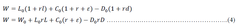
Where rl, r, and rd are determined variables, while ε is a form of a stochastic process and is normally distributed stochastic term with E(ε)=0. It is also assumed that ε is independent of all other variables in the model.

Following the model developed by Stoll (1978); Ho & Saunders (1981); McShane & Sharpe (1985); using Taylor's expansion, the bank's expectations of wealth at the end of the period, where E(W)=W¯, then the equation can be formulated as follows.

As a result of the same wealth expectations for each bank, the optimal NIM for each bank is assumed to be the same (Ho and Saunders, 1981). However, this assumption is not suitable in uncompetitive markets such as duopoly. If the behavior of the banking industry is assumed to be divided into two groups of banks – large bank and small bank – then each bank has a different expectation of its wealth. Therefore, loans and deposits must be estimated for each bank group that reaches an equilibrium condition. In the game theory framework, this equilibrium is called Nash equilibrium.

The type of game theory used in this study is the dynamic games of incomplete information. Furthermore, we use the Stackelberg model of duopoly (Gibbon, 1992), in which the decision making is sequential (dynamic), and the company is divided into two groups: the large (dominant) and the small (subordinate). In addition to dynamic elements, the use of game theory concepts in this study also includes elements of uncertainty. The game theory concept will generate NIM for each group of banks so that the optimal NIM generated will be close to the actual condition. The maximizing loan function of the large bank by using the game theory framework can be written in the equation below.

and the maximizing loan function for small bank is:

Where is constant from loan interest rate linear function, is a coefficient of loan interest rate linear function, r is the risk-free rate, and is a coefficient of the linear cost function for the loan.

The large and the small bank will maximize the deposit function using equations (8) and (9).

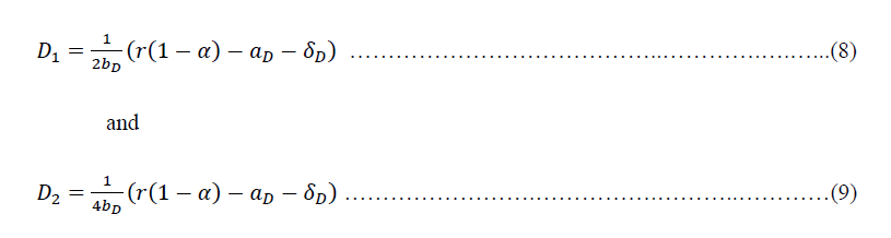
Where is constant from the linear interest rate deposit function, and is a coefficient of deposit interest rate linear function. The coefficient α is compulsory to reserve as a central bank policy instrument, and is a coefficient of the linear cost function for deposit. Therefore, we have two forms of bank wealth: the wealth for large banks and the wealth for small banks.

According to Ho & Saunders (1981); McShane & Sharpe (1985), the probability of getting bank deposits and loans is influenced by the movement of deposit and loan costs. Nevertheless, under the dynamic games of incomplete information framework, the probability of loans and deposits is not only influenced by the movement of loan and deposit costs. The probability of obtaining loans and deposits is also influenced by the uncertainty of the environment (nature) (Fudenberg & Tirole, 1992; Gibbon, 1992). The environment variables used in this study are the condition of economic growth (growth of Gross Domestic Product), which is positively linear in the probability of loans and deposits, and inflation, which is negatively linear with loans and deposits. Macroeconomic variables are believed to influence the demand for loans and deposits offerings within banking institutions (Cosimano & Hakura, 2011).

After mathematical derivation, the maximum NIM (spread) calculated based on the Ho & Saunders (1981) model by including the game theory conceptual framework for both large and small banks, the equations presented in (10) and (11).

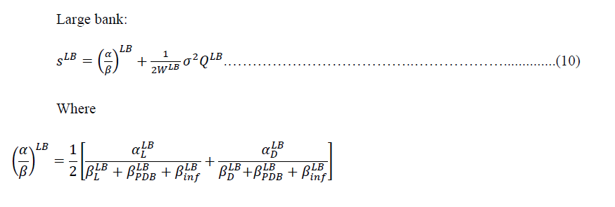
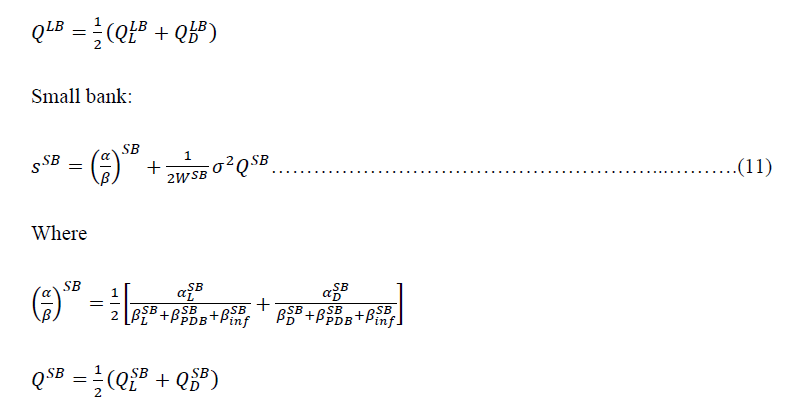
Models (10) and (11) resemble the Ho & Saunders (1981) models, but some components in the model have significant differences. The Ho and Saunders models that have been modified for the oligopoly market are divided into two models, the model for large banks and the model for small banks. Models (10) and (11) can be regarded as Ho and Saunders models, which have extended for the oligopoly market, where players do not cooperate (non-cooperative games) and consist of large banks and small banks with incomplete information. Models (10) and (11) are Ho and Saunders models for the dynamic game of incomplete information.

Additionally, the spreads in equations (10) and (11) are spreads (NIM) that reaches Nash equilibrium. Spreads that have reached Nash Equilibrium are payoffs for already optimal banks (Gibbon, 1992; Tirole, 1994). Banks that have spreads below the optimal value can increase their spreads until they reach the optimal amount, whereas banks that have spreads above the optimal value should reduce the spread to the optimal value.

To estimate optimal NIM using equations (10) and (11) we break down the equation into several parts so that some of its components can be obtained through linear equations, even though the overall model is not a linear model. The α and β values of each variable are obtained through linear equations, namely NIM as the dependent variable and the variable amount of loans, savings, economic growth, and inflation as the independent variable. Likewise with α and β in the loan and deposit functions in equations (6), (7), (8), and (9) all obtained by linear equations. Thus, some of these parameters are obtained through the panel data regression approach.

The empirical model used in this study follows the model used by Islam & Nishiyama (2016). The empirical equation used is as follows:

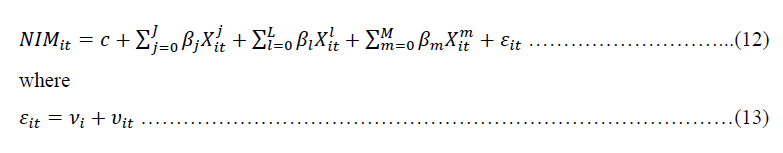
where _it is the net interest margin of bank i at time t where i = 1,. . .,N, t = 1,. . .,T and c is a constant variable. The superscripts j, l and m of X_it denote the bank-specific, industry specific and macroeconomic specific variables, respectively. is the disturbance with the unobserved bank-specific effect and the idiosyncratic error term. The error components of the regression model also distributed as IIN (0, ) and independent of IIN (0, ).

Alternative types of panel data models used are the Fixed Effect Model (FEM) and the Random Effect Model (REM). Pools Effect Model (PLS) / Common Effect Model are not used in this study because we consider this model does not reflect the characteristics of panel data as presented by Brooks (2008).

The Robustness Check

In addition to using the Risk Averse Dealer Model, this study also uses the One-Sample t-test to test the estimated NIM distribution during the observation period. One Sample t-test is used to test whether the optimal NIM of the estimation results is robust or not. The t-test model used is as follows (Gujarati & Porter, 2010):

where t is the value of the t distribution, is the sample mean, is the population mean, and is the standard deviation of sample.

Results and Discussion

This study extends the initial Ho and Saunders model using the game theory framework and the dynamic game of incomplete information. The determination of optimal NIM using the game theory framework follows equations (10) and equation (11). There are three scenarios used in determining optimal NIM using the game theory framework.

The first scenario involves 82 banks. There are 14 large banks (leader bank) and 68 small banks (follower bank) in the first scenario. The second scenario involves only 30 banks that have the same market, which represents nine economic sectors. In the second scenario, there are six large banks and 24 small banks, while the third scenario involves 62 banks, which are not included in the group of 30 banks, consisting of eight large banks and 54 small banks.

To obtain an optimal NIM (Nash Equilibrium) using the dynamic games of incomplete information approach as in equations (10) and (11), we used 16 variables in the equation. For the first scenario, the 16 values of these variables are presented in Table 6 below. All variables are estimated using panel data analysis and the random effect model.

Table 6 Parameter Value of 82 Banks Group
Parameter	Value	Sig.	R2
aL	0,5415	0,000	0.1380
bL	-0,0248	0,000
aD	0,1458	0,000	0.1848
bD	-0,0054	0,000
γL	0,7449	0,000	0.9637
δD	0,8728	0,000	0.9659
αLB	0,0355	0,005	0.5142
βγLB	0,2142	0,009
βδLB	0,3142	0,007
βegLB	0,0622	0,582
βinfLB	-0,0297	0,323
αSB	0,0325	0,000	0.4271
βγSB	0,1984	0,000
βδSB	0,1677	0,000
βegSB	0,1030	0,215
βinfSB	0,0790	0,017

Table 6 shows that from the 16 variables measured, three variables were not significant: economic growth and inflation rate in the large bank's group. Meanwhile, for the small bank group, only the economic growth variable was not significant. The R2 level varies for each variable, ranging from 0.1380 to 0.9659. The insignificant variable was not included in the estimation process.

Table 7 Parameter Value of Competitive Banks (30 BANKS)
Parameter	Value	Sig.	R2
aL	0,4460	0,000	0.1014
bL	-0,0187	0,001
aD	0,1450	0,000	0.3239
bD	-0,0057	0,000
γL	0,9459	0,000	0.9771
δD	0,8494	0,000	0.9788
αLB	0,0385	0,033	0.6321
βγLB	0,4790	0,009
βδLB	0,4363	0,000
βegLB	-0,3086	0,171
βinfLB	0,0187	0,657
αSB	0,0317	0,000	0.4758
βγSB	0,1891	0,000
βδSB	0,1739	0,000
βegSB	0,0951	0,184
βinfSB	0,0015	0,937

The parameter values for the second scenario, namely the 30 banks (competitive bank) presented in Table 7. In the second scenario, namely the group of 30 banks (competitive bank), it is known that there are four insignificant variables, where two variables are for large banks and small banks. The insignificant variables were economic growth and the inflation rate for both large and small bank groups. At the same time, the value of R2 varies between 0.1014 to 0.9788.

The parameter values used to estimate the bank NIM that reaches Nash Equilibrium in the third scenario (specific bank) can be seen in Table 8 below. The R2 value varies between 0.1215 to 0.9435. Of the 16 variables estimated, three variables are not significant, two variables in the large bank group and one variable in the small bank group. The variables that do not affect the large bank groups are economic growth and the inflation rate. Meanwhile, the variable that does not affect the small bank group is the Saving Service Fees (δ).

Table 8 Parameter Value of Specific Banks (62 BANKS)
Parameter	Value	Sig.	R2
aL	0.59	0,000	0.1215
bL	-0.0277	0,000
aD	0.1754	0,004	0.1517
bD	-0.0075	0,069
γL	0.91	0,000	0.9435
δD	0.92	0,000	0.9412
αLB	0.02059	0,012	0.4995
βγLB	0.33063	0,000
βδLB	0.43439	0,000
βegLB	0.07345	0,531
βinfLB	0.01615	0,658
αSB	0.03624	0,000	0.2669
βγSB	0.12217	0,000
βδSB	0.05096	0,056
βegSB	0.17452	0,041
βinfSB	0.10451	0,000

Based on the game theory framework, the optimal NIM level for large bank groups is relatively stable at around 6.721 per cent to 6.969 per cent. While the average of optimal NIM for large banks is about 6.78 per cent, this value is higher than 0.96 per cent compared to the average of actual NIM of large banks, which was 5.82 per cent.

Table 9 The Optimal Nim Using Game Theory For Large Bank And Small Bank, Group Of 82 Banks (%)
Year	Optimal NIM of Large Bank	Optimal NIM of Small Bank	Average Actual NIM of Large Bank	Average Actual NIM of Small Bank	Deviation of Large Bank	Deviation of Small Bank
2008	6.760	7.317	6.515	7.045	-0.24	-0.27
2009	6.969	7.327	6.312	6.748	-0.66	-0.58
2010	6.721	7.306	5.886	6.713	-0.83	-0.59
2011	6.732	7.308	5.744	6.353	-0.99	-0.96
2012	6.722	7.306	5.712	5.995	-1.01	-1.31
2013	6.776	7.324	5.615	6.154	-1.16	-1.17
2014	6.722	7.306	5.539	5.764	-1.18	-1.54
2015	6.722	7.306	5.520	5.574	-1.20	-1.73
2016	6.890	7.339	5.857	5.890	-1.03	-1.45
2017	6.738	7.308	5.501	5.586	-1.24	-1.72
AVERAGE	6.775	7.315	5.820	6.182	-0.96	-1.13

These results indicate that the average NIM level of large banks in Indonesia has not yet reached its optimal level. The result indicates that large banks in the first group still have the potential to increase their profitability. Large banks can increase their profitability by increasing their NIMs to the optimal level of 6.78 per cent.

The optimal NIM for small banks is relatively stable, around 7.32 per cent, with a range between 7.31 per cent and 7.34 per cent. The optimal NIM of small banks is higher than the actual NIM, which has only reached 6.18 per cent. The deviation of optimal NIM and the actual NIM is around 1.13 per cent, and the optimal NIM is higher than the actual NIM.

Similar to large banks, small banks in the Indonesian banking industry still have the potential to increase their profits. They can increase the actual NIM by 1.13 per cent to attain an optimal NIM. Thus, in the Indonesian banking industry, both large and small banks in the first scenario each have the opportunity to raise their NIM levels.

However, increasing bank NIMs presents a trade-off effect. The positive impact is that raising the NIM can increase bank profits. However, on the other hand, for regulators, this is not a good condition. An increase in bank NIM will have an impact on high loan interest rates that may result in a high-cost economy and slow down economic growth.

We also perform a robustness check for the estimation by testing whether the bank's optimal NIM (Nash Equilibrium) value is equal to the average optimal NIM during the observation period. We use One-Sample t-test model to check the optimal NIM from estimation. The model has been described in equation (14).

Table 10 One Sample T-Test For Optimal Nim of Large Bank – Small Bank Group of 82 Banks
	t-value	Sig. (2-tailed)
Optimal NIM of Large Bank	1.303	0.225
Optimal NIM of Small Bank	-1.436	0.185

The observation used was the t-test with the one sample t-test approach, as shown in Table 10 above. The results indicate that the average optimal NIM of large and small banks in a group of 82 banks is not different from the optimal NIM of banks each year. The significance value of the one sample t-test on the large and small bank groups is greater than 0.05, so the hypothesis that the optimal NIM of Game Theory in the 82 banks group is consistent during the research period.

Table 11 provides the results of the second scenario that consists of 6 large banks and 24 small banks.

Table 11 The Optimal Nim Using Game Theory For Large Bank And Small Bank, Group Of 30 Banks (%)
Year	Optimal NIM of Large Bank	Optimal NIM of Small Bank	Average Actual NIM of Large Bank	Average Actual NIM of Small Bank	Deviation of Large Bank	Deviation of Small Bank
2008	4.209	8.734	6.50	5.65	2.29	-3.09
2009	4.211	8.736	6.33	5.90	2.12	-2.84
2010	4.206	8.732	6.61	4.99	2.40	-3.74
2011	4.206	8.732	6.33	5.25	2.12	-3.49
2012	4.206	8.732	6.22	5.36	2.02	-3.37
2013	4.210	8.736	6.25	5.14	2.04	-3.60
2014	4.206	8.732	6.21	4.77	2.00	-3.96
2015	4.206	8.732	6.20	4.83	2.00	-3.90
2016	4.214	8.739	6.29	4.96	2.07	-3.78
2017	4.206	8.732	5.91	4.71	1.70	-4.03
AVERAGE	4.208	8.733	6.28	5.15	2.07	-3.58

In the second scenario, the optimal NIM for large banks is 4.21 per cent, while the average of the actual NIM of large banks is 6.28 per cent. The deviation between actual NIM and optimal NIM for the large banks group is around 2.08 per cent. The results imply that a bank large should reduce the actual NIM level to reach the optimal NIM. This step will be mutually beneficial both for banks and for regulators (government). For banks, even though the NIM is down, this step will increase the demand for loans to the bank group and thus increase the bank's profit. On the other hand, the government will also benefit because loan interest rates will decline. The decrease in loan interest rates will be followed by company expansion through bank loans. Increased business expansion will encourage national economic growth.

The results also indicate that small banks still have a chance to increase their NIMs. Small banks can increase their NIMs by up to 3.58 per cent. For small banks, this step will certainly be very profitable. However, for the government, this step will hinder national economic growth due to a large number of small banks.

While the optimal NIM for the small bank group is around 8.73 per cent, the average actual NIM of the small bank group is around 5.15 per cent. The actual NIM of small banks is still lower than the optimal NIM.

In the second scenario, the results of the one sample t-test also show that the average NIM from the estimation of the Game Theory approach has the same magnitude (stable). Thus, it can be concluded that the NIM estimation results of Game Theory is robust.

The results of the one sample t-test for large and small banks in the second scenario (group of 30 banks) show that the data is robust because the optimal bank NIM average is statistically the same during research period. The results of the one sample t-test can be seen in Table 12 below.

Table 12 One Sample T-Test For Optimal Nim Of Large Bank – Small Bank Group Of 30 Banks
	t-value	Sig. (2-tailed)
Optimal NIM of Large Bank	-2.206	0.055
Optimal NIM of Small Bank	0.887	0.398

In the last scenario, the banks are assumed to be unique and only focus on specific market segments. Banks in this group are assumed to have monopoly power in particular markets so that they can influence the actual NIM rate prevailing in the market. Based on the third scenario, the average optimal NIM for large banks is 2.75 per cent, and the average of actual NIM of large banks is 5.47 per cent. This finding demonstrates that those banks need to reduce the actual NIM by 2.72 per cent to reach the optimal level.

Table 13 The Optimal Nim Using Game Theory For Large Bank And Small Bank, Group Of 62 Banks (%)
Year	Optimal NIM of Large Bank	Optimal NIM of Small Bank	Average Actual NIM of Large Bank	Average Actual NIM of Small Bank	Deviation of Large Bank	Deviation of Small Bank
2008	2.760	9.090	6.53	7.51	3.768	-1.584
2009	3.226	9.918	6.30	6.99	3.071	-2.926
2010	2.691	9.033	5.35	7.27	2.654	-1.767
2011	2.751	9.044	5.30	6.65	2.553	-2.391
2012	2.700	9.034	5.33	6.18	2.628	-2.853
2013	2.961	9.195	5.14	6.40	2.179	-2.797
2014	2.693	9.034	5.03	6.01	2.341	-3.021
2015	2.705	9.034	5.01	5.76	2.304	-3.278
2016	2.329	9.205	5.53	6.15	3.206	-3.051
2017	2.680	9.046	5.19	5.85	2.514	-3.200
AVERAGE	2.750	9.163	5.47	6.48	2.722	-2.683

The reduction in NIMs of large banks in this group will certainly make the government happy, because it will push loan interest rates lower to encourage economic growth. Also, the number of large banks in this group is quite large – eight banks – so the economic multiplier effect will be more significant. While the average optimal NIM for small banks in this last scenario is 9.16 per cent, this amount is higher than the actual average small bank NIM, which is 6.48 per cent. The difference between the actual NIM and the optimal NIM is 2.68 per cent.

The results of this study indicate that small banks in the specific bank group have not utilized their market power optimally. With their market power, these banks have the potential to increase profits by increasing NIMs. Small banks in the specific bank group can increase their NIMs by 2.68 per cent to achieve an optimal NIM.

Nevertheless, the increase in NIM in this small bank group will make the government very dissatisfied. The increase in NIM in the small bank group can significantly impact the condition of the national economy because the number of small banks in this group is enormous, 54 banks. The increase in NIMs will result in a significant increase in loan interest rates among these small banks and will create a high-cost economy in the Indonesian economy.

Similar to the robust test results in the first and second scenarios, the results of the one sample t-test for large and small banks in the third scenario for specific banks (group of 62 banks) show that the data is robust because the average optimal bank NIM is statistically the same during the research period. The result of the one sample t-test is more clearly seen in Table 14.

Table 14 One Sample T-Test For Optimal Nim Of Large Bank – Small Bank Group Of 62 Banks
	t-value	Sig. (2-tailed)
Optimal NIM of Large Bank	-0.006	0.996
Optimal NIM of Small Bank	0.003	0.997

Table 15 summarizes the results of the NIM bank from the estimation of the Game Theory model. Estimation results show that in the first group (involving all banks), large banks and small banks have an average actual NIM that is still below their optimal value (under optimal). In the competitive bank group, large banks have an actual NIM above their optimal NIM (over optimal), whereas small banks have actual NIMs that are smaller than their optimal NIMs. In the specific bank group, large banks still have an actual NIM that is above the optimal NIM, whereas small banks have actual NIMs that are smaller than their optimal NIMs.

Table 15 Summary Result Of Nim From Game Theory Estimation
Group	Large Bank	Small Bank
All Bank	Under Optimal	Under Optimal
Competitive Bank	Over Optimal	Under Optimal
Specific Bank	Over Optimal	Under Optimal

For banks with an actual NIM less than the optimal NIM, the bank still has the opportunity to increase the actual NIM up to the optimal NIM. Whereas a bank with an actual NIM is higher than its optimal NIM, the bank should lower its actual NIM level so that the actual NIM is the same as the optimal NIM. From the results of this study note that all small banks in all bank groups have an actual NIM that is smaller than the optimal NIM. Small banks still have a chance to raise their NIMs to the optimal NIMs.

These results differ from those of Sidabalok & Viverita (2011); Rosengard & Prasetyantoko (2011); Trinugroho et al., (2014); Abdullah et al., (2016). They concluded that the NIM of banks in Indonesia was too high, which resulted in inefficient banks' performance in Indonesia. According to their research, the NIM of banks in Indonesia is the highest among the big five ASEAN Countries and must be lowered.

The difference in the results of this study is caused by differences in the concepts and methods used. They still use the concept of The Initial Risk-Averse Dealer Model, although with different methods. Sidabalok and Viverita use dynamic panel data in estimating bank NIM. Rosengard & Prasetyantoko (2011) used descriptive analysis to determine the average NIM level in the Indonesian banking industry. While Trinugroho et al., (2014) estimate an econometric model using a pooled regression and static and dynamic panel regressions. Abdullah et al., (2016) use the Game Theory approach, but they estimate bank lending rates, not NIM.

However, this study found that there is still room for some banks to increase their NIM levels. Our conclusion is based on several conditions, namely the condition of environmental uncertainty, the financial condition of the company, and the condition of competition between banks (market structure). Based on these considerations and the company viewpoint, the actual NIM of banks in Indonesia is not too high, and even banks still have a chance to increase their NIM.

Conclusion

This study extended the Ho & Sounders (1981) to determine banks NIM in an uncompetitive market structure. By using the game theory framework, banks can determine the optimal NIM level. Furthermore, this study divided the sample bank into two groups, large banks as lead banks and small banks as follower banks. The study also segregates the sample into three scenarios based on the market condition. Using the extended model in the Indonesian banking sector, we find that the group of small banks always has an optimal NIM that is higher than their actual NIM in all scenarios. In contrast, large bank groups have an optimal NIM greater than the actual NIM only in the first scenario. In the second and third scenarios, the optimal NIM of a large bank group is always lower than the average actual NIM.

Results of these study impact two institutions at the same time, banks and the government, but with different effects. For most banks, the results of this study can be a justification for increasing their NIM to increase the level of bank profitability. Most large banks, namely large banks in the first scenario group, can raise their NIMs to the optimal level. In contrast, large banks in the second and third scenario groups must reduce their NIM level because the actual NIM is higher than the optimal NIM, and small bank groups in all scenarios still can increase profits by increasing their NIM levels. This is because the actual NIM of a small bank is still smaller than the optimal NIM.

Nevertheless, the result may problematic for the government. An increase in bank NIMs will increase the interest rate that can cause reduces the loan demand. The company will delay the expansion of its business and thus slow economic growth. In the end, the increase in bank NIM can result in a high-cost economy in the Indonesian economic system.

Despite its contribution, this study has some limitations. For example, it might be useful to compare the results using different assumptions and methods. As explained before, this study only focuses on game theory types of dynamic games of incomplete information. Thus, it cannot identify the optimal NIM using other game theory models, such as static games of complete information, dynamic games of complete information, and static games of incomplete information.

Acknowledgement

This paper is a part of a dissertation that is being prepared by the author at the Department of Management, Faculty of Economics and Business, Universitas Indonesia.

References

Abdullah, P., Bary, P., Khasananda, R., & Sya’banni, R.E. (2016). Competition leader-follower interaction: Panel estimates on Indonesia banking. Bulletin of monetary and banking economics, 19(1), 22–38.

Crossref , Google Scholar , Indexed

Adita, C., & Kusuma, C. (2015). The dynamics of Indonesian banking competition 2006 – 2013. Building Economy 19(1), 26 – 420.

Crossref , Google Scholar

Allen, L. (1988). The determinant of bank interest margins: A note. The Journal of Financial and Quantitative Analysis 23(2), 231 – 235.

Crossref , Google Scholar , Indexed

Angbazo, L. (1997). Commercial bank net interest margin, default risk, interest-rate risk, and off-balance sheet banking. Journal Banking and Finance, 21, 55 – 87.

Crossref , Google Scholar , Indexed

Beck, T., Demirguc-Kunt, A., & Maksimovic, V. (2004). Bank competition and access to finance: International evidence. Journal of Money, Credit, and Banking 36(3), 627 – 648.

Crossref , Google Scholar , Indexed

Beck, T., & Hesse, H. (2009). Why are interest spread so high in Uganda?. Journal of Development Economics, 88, 192 – 204.

Crossref , Google Scholar , Indexed

Berger, A.N. (1995). The profit-structure relationship in banking-tests of market-power and efficient-structure hypotheses. Journal of Money, Credit and Banking, 27(2), 404 – 431.

Crossref , Google Scholar , Indexed

Berger, A.N., Molyneux, P., Wilson, J.O.S. (2020). Banks and the real economy: An assessment of the research. Journal of Corporate Finance, 62, 1 – 14.

Google Scholar , Indexed

Chen, S.H., Liao, C.C. (2011). Are foreign banks more profitable than domestic banks? Home – and host-country effect on banking market structure, governance, and supervision. Journal of Banking and Finance, 35, 819 – 839.

Crossref , Google Scholar , Indexed

Church, J., Ware, R. (2000). Industrial organization. A Strategic Approach. MCGraw-Hill. United State of America.

Crossref , Google Scholar , Indexed

Cosimano, T.F., & Hakura, D. (2011). Bank behavior in response to Basel III: A cross-country analysis. IMF Working Paper No. 11/119.

Crossref, Indexed

Drakos, K. (2003). Assessing the success reform in transition banking10 years later: An interest margin analysis. Journal of Policy Model, 25, 309 – 317.

Entrop, O., Memmel, C., Ruprecht, B., &Wilkens, M. (2015). Determinant of bank interest margin: Impact of maturity transformation. Jurnal of Banking and Finance, 54, 1 – 19.

Freixas, X., & Rochet, J.C. (2008). Microeconomics of Banking, (Second Edition). The MIT Press. London, England

Crossref , Google Scholar , Indexed

Fudenberg, D., & Tirole, J. (1992). Game Theory. The MIT Press. Cambridge, England.

Crossref , Google Scholar , Indexed

Gibbons, R. (1992). Game theory for applied economists. Princeton University Press. New Jersey

Goddard, J., Liu, H., Molyneux, P., Wilson, J.O.S. (2011). The persistence of bank profit. Journal of Banking and Finance, 35, 2881-2890.

Gujarati, DN., & Porter, D.C. (2010). Essentials of econometrics, (Fourth Edition). McGraw-Hill/Irwin. United States

Ho, T.S.Y., Saunders, A. (1981). The determinant of bank interest margin: Theory and empirical evidence. The Journal of Financial and Quantitative Analysis, 16, 581 – 600.

Crossref , Google Scholar , Indexed

Huck, S., Konrad, K.A., & Muller, W. (2001). Big fish eat small fish: On merger Stackelberg market. Economics Letters, 73, 213 – 217.

Crossref , Google Scholar , Indexed

Islam, M.S., & Nishiyama, S.I. (2016). The determinant of bank net interest margin: A panel evidence from South Asia countries. Research in International Business and Finance, 37, 501 – 514.

Crossref , Google Scholar , Indexed

Kasman, A., Tunc, G., Vardar, G., & Okan, B. (2010). Consolidation and commercial bank net interest margins: Evidence from the old and new European Union members and candidate countries. Economic Modelling, 27, 648 – 655.

Crossref , Google Scholar , Indexed

Khawaja, M.I., & Din, M. (2007). Determinant of interest spread in Pakistan. The Pakistan development review, 46(2), 129 – 143.

Google Scholar , Indexed

Klein, M. (1971). A theory of the banking firm. Journal of Money, Credit, and Banking, 3, 205 – 218.

Crossref , Google Scholar , Indexed

Kunt, A.D., Huizinga, H. (1999). Determinant of commercial bank interest margin and profitability: Some International evidence. The World Bank Economic Review, 13(2), 379 – 408.

Crossref , Google Scholar , Indexed

Lopes-Espinosa, G., Moreno, A., & de Gracia, F.P. (2011). Banks’ net interest margin in the 2000s: A macro-accounting international perspective. Journal of International Money Finance, 30, 1214 – 1233.

Crossref , Google Scholar , Indexed

Maudos, J., & Solis, L. (2009). The determinant of net interest income in the Mexican banking system: An integrated model. Journal of Banking and Finance, 33, 1920 – 1931.

Crossref , Google Scholar , Indexed

McShane R.W., & Sharpe, L.G. (1985). A time series / cross section analysis of the determinants of Australian trading bank loan / deposit interest margins: 1962 – 1982. Journal of Banking and Finance, 9, 115 – 136.

Crossref , Google Scholar , Indexed

Michaelsen, J.B., & Goshay, R.C. (1967). Portfolio selection in financial intermediaries: A new approach. The Journal of Financial and Quantitative Analysis, 2(2), 166 – 199.

Crossref , Google Scholar , Indexed

Mirzaei, A., Moore, T., & Liu, G. (2013). Does market structure matter on banks’ profitability and stability? Emerging vs. advanced economies. Journal of Banking & Finance, 37, 2920 – 2937.

Crossref , Google Scholar

Monti, M. (1972). Deposit, credit, and interest rate determination under alternative bank objectives. In Mathematical methods in investment and finance, (edition). G. P. Szego and K. Shell. Amsterdam: North Holland.

Indexed

Niu, C., Guo, X., Wang, T., & Xu, P. (2014). Regret theory and the competitive form: A comment. Economic Modelling, 41, 312 – 315.

Crossref , Google Scholar , Indexed

Pyle, D.H. (1972). Descriptive theories of financial institution under uncertainty. The Journal of Financial and Quantitative Analysis, 7(5), 2009 – 2029.

Crossref , Google Scholar , Indexed

Rosengard, J.K., Prasetyantoko, A. (2011). If the banks are doing so well, why can’t I get a loan? Regulatory constraints to financial inclusion in Indonesia. Asian Economic Policy Review, 6, 273 – 295.

Crossref , Google Scholar , Indexed

Saksonova, S. (2014). The role of net interest margin in improving banks’ asset structure and assessing the stability and efficiency of their operations. Social and Behavioral Sciences, 150, 132 – 141.

Crossref , Google Scholar , Indexed

Sauer, C., & Scheide, J. (1995). Money, interest rate spread, and economic activity. Weltwirtschaftliches Archiv, 131(4), 708 – 722.

Crossref , Google Scholar , Indexed

Saunders, A., & Schumacher, L. (2000). The determinant of bank interest margin: An international study. Journal of International Money and Finance, 19, 813 – 832.

Crossref , Google Scholar

Sensarma, R., & Ghosh, S. (2004). Net interest margin: Does ownership matter? Vikalpa, 29(1), 41 – 47.

Crossref , Google Scholar , Indexed

Sidabalok, S.R., & Viverita, V. (2011). The determinant of net interest margin in the Indonesian banking sector.

Crossref , Google Scholar , Indexed

Daryanto, S.A., Arifin, B., & Priyarsono, D.S. (2011). Market Structure of Indonesian Banking Competition in the Consolidation Period. Journal of Management and Agribusiness, 8(2), 115 – 128.

Tarus, D.K., Chekol, Y.B., & Mutwol, M. (2012). Determinants of net interest margins of commercial banks in Kenya: A panel study. Procedia Economics and Finance, 2, 199 – 208.

Crossref , Google Scholar , Indexed

Tirole, J. (1994). The theory of industrial organization. The MIT Press. London, England.

Trinugroho, I., Agusman, A., & Tarazi, A. (2014). Why have bank interest margins been so high in Indonesia since the 1997/1998 financial crisis?. Research in International Business and Finance, 32, 139-158.

Crossref , Google Scholar , Indexed

Tsai, J.Y. (2013). Bank interest margin management based on a path-dependent Cobb-Doglas utility framework. Economic Modelling, 35, 751 – 762.

Crossref , Google Scholar , Indexed

Vilverde, C.S., & Fernandez, F.R. (2007). The determinant of bank margins in European banking. Journal of Banking and Finance, 31, 2043 – 2063.

Crossref , Google Scholar , Indexed

Wibowo, B. (2017). Banking competition measurement and banking sector performance: Analysis of 4 ASEAN Countries. Journal of Economics, 6(1), 1 – 28.

Crossref , Google Scholar , Indexed

Widyastuti, R.S., & Armanto, B. (2013). Banking industry competition in Indonesia. Bulletin of Monetary, Economics and Banking, 401 – 434.

Crossref , Google Scholar , Indexed

Wong, K.P. (2014). Regret theory and competitive firm. Economic Modelling, 36, 172–175.

Crossref , Google Scholar , Indexed

Wong, K.P. (2011). Regret theory and the banking firm: The optimal bank interest margin. Economic Modelling, 28, 2483 – 2487.

Crossref , Google Scholar , Indexed

Wong, K.P. (1997). On the determinants of bank interest margins under credit and interest rate risk. Journal of Banking and Finance, 21, 251 – 271.

Crossref , Google Scholar , Indexed

Wu, PC., Liu, S.Y., & Zhai, R.X. (2018). Nonlinear impacts of operating risk and demand management policy on banks’ performance: The role of leading indicator. Economic Analysis and Policy, 59, 40 – 53.

Crossref , Google Scholar , Indexed

Zarruk, E.R. (1989). Bank spread with uncertain deposit level and risk aversion. Journal of Banking and Finance, 13, 797 – 810.

Crossref , Google Scholar , Indexed

Zarruk, E.R., & Madura, J. (1992). Optimal bank interest margin under capital regulation and deposit insurance. The Journal of Financial and Quantitative Analysis, 27(1), 143 – 149.

Crossref , Google Scholar , Indexed

Zhou, K., & Michael, C.S.W. (2008). The determinant of net interest margin of commercial bank in Mainland China. Emerging Markets Finance and Trade, 44(5), 41 – 53.

Crossref , Google Scholar , Indexed

Received: 29-Dec-2021, Manuscript No. AAFSJ-21-5196; Editor assigned: 01-Jan-2021, PreQC No. AAFSJ-21-5196(PQ); Reviewed: 12-Jan-2021, QC No. AAFSJ-21-5196; Revised: 22-Jan-2022, Manuscript No. AAFSJ-21-5196(R); Published: 29-Jan-2022