Keywords

Macroeconomic Forecasts; Expert Adjustment.

Introduction

We evaluate the quality of individual forecasts from Consensus Economics Inc., where the forecasts concern growth in Gross Domestic Product (GDP), the inflation rate (CPI-based) and the unemployment rate, all for the USA. These forecasts have been analysed before in various studies. An example is Isiklar and Lahiri (2007) who analyse the quality of the forecasts over various horizons. Batchelor (2007) examines the bias in the forecasts, while Dovern and Weisser (2011) additionally look at accuracy and efficiency of the individual forecasts. As the Consensus forecasts are usually created each month for next year’s economic entity, Isiklar, Lahiri and Loungani (2006) examine forecast revisions, whereas Batchelor (2001) and Loungani (2001) consider various other features of the professional forecasts from Consensus. Other relevant studies that compare and combine individual forecasters are D’Agostino et al. (2010), Genre et al. (2013) and Bürgi & Sinclair (2017).

In this paper we also zoom in on the properties of the individual Consensus forecasters and our angle is that we want to understand what it is that these forecasters actually do and why some individual forecasters perform better than others. Indeed, although we do have forecasts and realizations, we are usually unaware of what it could be that these forecasters do when they create their forecasts. So, could more forecast accuracy just be a lucky draw? Or, can we discern strategies that lead to better performance. One recent study that aims at related aspects is the study of Frenkel, Ruelke and Zimmermann (2013), where it is analysed if forecasters intentionally deviate from forecasts from the IMF or OECD once these become available. Here, we focus on something similar, with one key difference. As we do not know how exactly IMF or OECD forecasts themselves are created, which also allows for the possibility that the IMF and OECD forecasters in turn look at past Consensus forecasts, we decide to create our own benchmark model-based forecasts ourselves. These benchmark forecasts are based on simple time series averages and with these we can assume that the observed individual Consensus forecasts are so-called expert-adjusted forecasts. Indeed, the benchmark forecasts are simple moving averages of the most recent and available realizations of GDP growth, inflation and unemployment and so it is reasonably safe to assume that any forecaster could have used these as a benchmark model forecast too. When we interpret the individual Consensus forecasts as expert-adjusted forecasts, we can now draw on various findings in the recent literature on expert-adjusted forecasts. Franses (2014) summarizes various theoretical results on how optimal expert-adjusted forecasts could look like. With these, we can assign behavioural aspects to the Consensus forecasters and in a next step we correlate these behavioural features with actual performance. This latter correlation thus allows us to examine why some forecasters do better than others and if good or poor performance is just luck or bad luck.

The outline of our paper is as follows. In Section 2 we present the accuracy of the individual Consensus forecasts relative to each other and relative to the simple benchmarks. The main conclusion here is that there is quite some variation in performance. Note that this is not necessarily a bad sign, see Zarnowitz and Lambros (1987), Lahiri and Sheng (2010) and recently Legerstee and Franses (2015) who show that also disagreement can have predictive value. In Section 3 we create indicators of the behaviour of the professional forecasters and we correlate these indicators with their individual forecast accuracy. In Section 4 we provide various conclusions and we also suggest avenues for further research.

The Forecasts and Their Accuracy

We collect the forecasts for yearly values of GDP growth, the inflation rate and the unemployment rate from Consensus Economics Inc. We have forecasts created in the months of 2000M01 to and including 2013M12 and we have realizations of the annual data for 2001 to 2014 (retrieved May 2015). The maximum number of monthly forecasts is thus 14 times 12 is 168. Each forecast can be viewed as an update, but in this paper we do not focus on forecast revisions, but merely we compare the monthly forecasts for next year’s economic entity with its actual realization in that particular year. Later we will create benchmark model-based forecasts.

Forty Professional Forecasters

First, we focus on the professional forecasters in our sample. Table 1 report their names or institutions and the number of forecasts they have provided in the sample period of interest. DuPont gave forecasts in all 168 months, while we decide to include Mortgage Bankers Assoc. with their 36 forecasts as a minimum of three years of data. Below we will need these 36 observations in regression models and hence we do not include other forecasters with smaller amounts of forecasts. It should be stressed that not all provided forecasts concern connected observations and for many of the 40 forecasters there are gaps in their reporting. Figure 1 shows a histogram of the data in Table 1 and clearly there is quite some variation in inclusion in each month’s panel of forecasts. This implies that the average Consensus forecast that is so often used rarely concerns an average of the quotes of the very same professional forecasters. This is not necessarily a bad sign, it is just a fact.

Table 1: The professional forecasters included in consensus economics inc. And the Number Of Forecasts Available In Our Sample (2000m01-2013m12)
Forecasters	Number of forecasts
	GDP	CPI	UR
DuPont	168	168	168
Inforum - Univ of Maryland	162	162	162
JP Morgan	162	162	162
Eaton Corporation	157	156	157
Nat Assn of Home Builders	153	153	153
The Conference Board	153	153	153
Fannie Mae	151	151	151
General Motors	151	151	151
Wells Capital Mgmt	149	149	149
Goldman Sachs	148	148	148
Univ of Michigan - RSQE	148	148	148
Ford Motor Corp	146	143	146
Oxford Economics	146	146	146
Macroeconomic Advisers	144	143	143
Morgan Stanley	142	142	142
Georgia State University	135	135	135
Merrill Lynch	110	110	110
Daimler Chrysler	105	105	104
Bank America Corp	100	100	100
Credit Suisse	98	98	98
Econ Intelligence Unit	98	98	97
Swiss Re	88	88	88
Standard & Poor's	85	85	85
Wachovia Corp	82	82	82
Lehman Brothers	80	80	80
Northern Trust	70	70	70
Global Insight	63	63	63
Bear Stearns	60	59	59
United States Trust	58	57	56
Economy.com	56	56	56
Wells Fargo	53	53	53
First Trust Advisors	51	51	51
Moody's Economy.com	49	49	49
Barclays Capital	48	48	48
IHS Global Insight	47	47	47
Prudential Financial	44	44	44
RDQ Economics	43	43	43
Bank of America - Merrill	42	42	42
Bank One Corp	37	35	37
Mortgage Bankers Assoc	36	36	36

In Table 2 we present the accuracy of the forecasts for the three variables where we rely on four criteria. These criteria are the Mean Squared Error (MSE), the Root MSE, the Mean Absolute Error (MAE) and the Mean Absolute Scaled Error (MASE). The latter criterion¹ is particularly advocated in Hyndman and Koehler (2006) and Franses (2016).

Table 2: Accuracy Of Forecasts From 40 Forecasters, Based On Four Different Accuracy Measures
	Mean	Median	SD	Minimum	Maximum
GDP
MSE	3.874	4.091	2.362	0.621	13.508
RMSE	1.878	2.023	0.596	0.788	3.675
MAE	1.333	1.354	0.401	0.612	2.847
MASE	0.770	0.782	0.232	0.353	1.645
Inflation rate
MSE	1.376	1.329	0.490	0.548	2.829
RMSE	1.156	1.153	0.204	0.740	1.682
MAE	0.904	0.901	0.190	0.554	1.480
MASE	0.810	0.808	0.171	0.497	1.327
Unemployment rate
MSE	1.071	1.147	2.818	0.164	2.818
RMSE	0.986	1.070	0.319	0.405	1.679
MAE	0.658	0.680	0.174	0.344	1.167
MASE	0.799	0.826	0.211	0.419	1.417

The numbers in Table 2 show that the forecasts for GDP growth can be pretty poor. On average the mean absolute error is 1.333, which, given the usual scale of GDP growth, is quite large. At the same time, the variation in the forecast quality is also substantial. The maximum RMSE is as large as 3.675. For inflation and unemployment the variation in accuracy is smaller than for GDP. Apparently, these first two variables are easier to predict than GDP growth. The main take-away from Table 2 is that there is substantial variation in forecast performance across the 40 individual forecasters.

Table 3 reports the top five performing forecasters. Note that the rankings for MSE and RMSE are necessarily the same and this of course also holds for MAE and MASE. Across the criteria, we see similar rankings for each variable. In contrast, across the three variables we see different top five rankings. Hence, forecasters with high accuracy for GDP growth do not necessarily perform well for the other two variables and the other way around.

Table 3: Best Performing Forecasters (Standard Deviations Are Not Taken Into Account)
		GDP	Inflation	Unemployment
	MSE/RMSE
Rank	1	Economy.com	Prudential Financial	RDQ Economics
	2	Wells Fargo	Bank One Corp	Mortgage Bankers
	3	IHS Global Insight	IHS Global Insight	United States Trust
	4	Bank of America – Merrill	Mortgage Bankers	Barclays Capital
	5	Barclays Capital	RDQ Economics	Standard & Poor’s
	MAE/MASE
Rank	1	Economy.com	Bank One Corp	United States Trust
	2	Wells Fargo	IHS Global Insight	Barclays Capital
	3	IHS Global Insight	Prudential Financi	RDQ Economics
	4	Barclays Capital	Credit Suisse	Mortgage Bankers
	5	Bank of America-Merrill	Mortgage Bankers	Standard & Poor’s

The forecasters rated in Table 3 seem to appear in the bottom end of Table 1, thereby suggesting that those forecasters who only quote a small amount of forecasts could perform better. To see if there might be an overall connection between the number of quotes and accuracy, consider for example Figure 2. Here we present a scatter of the MSE for GDP forecasts against the number of quotes and clearly there does not seem much of a correlation. For the other accuracy measures and the other variables we get similar scatters. Below we will examine if other indicators of behaviour can perhaps better explain forecast performance.

Benchmark Forecasts

We now turn to the creation of a model-based benchmark forecast. This forecast should potentially be publicly available to each of the professional forecasters. Hence, basically, it should therefore be a simple summary of the most recent publicly available observations on the variables of interest. As we often see in practice that the no-change forecast (sometimes called the random walk forecast) is hard to beat, we decide to employ the average value of the three most recent observations in the monthly data. For inflation and the unemployment rate, these observations are indeed available at the monthly level, whereas for GDP growth only quarterly data are available. This means that for each month t and variable y_t, we consider the forecast for the next year as 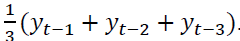When the data are quarterly, we use for the lagged y_t those data that are available at that time. Naturally, this model-based forecast can be improved along many dimensions, for example by including the past of the other two variables and by including even many more other economic indicators. However, in all those cases, subjective judgments have to be made by the professional forecasters or by an analyst and as such, by just taking an average of the last three months, we can assume that all forecasters could have equally used this “model-based” forecast as their input for their own forecast. Now, given the availability of a model-based forecast, we can thus interpret the professional forecasts as expert-adjusted forecasts and we can use various metrics of the differences between the model-based forecasts and the expert-adjusted forecasts as indicators of individual behaviour.

Before we turn to those indicators of behaviour, we first provide some accuracy measures of the benchmark forecasts in Table 4. Not surprisingly, the quality of the three-months average forecast is not very good, for any of the three variables of interest. In particular for CPI inflation the benchmark performs worse than any of the 40 forecasters.

Table 4: Benchmark Forecasts And Their Forecast Accuracy
Variable	Criterion	Score
GDP	MSE	6.791
	RMSE	2.606
	MAE	2.047
	MASE	1.183
Inflation rate	MSE	8.894
	RMSE	2.982
	MAE	2.085
	MASE	1.869
Unemployment rate	MSE	2.083
	RMSE	1.443
	MAE	0.988
	MASE	1.201

In Table 5 we report the relative scores of the accuracy measures, that is, we divide for example the MSE of each of the forecasters by the MSE of the benchmark model and then take the average. A score of 1 signal that they are equally good; while a score below 1 means that the professional forecasters are more accurate. From Table 5 we learn that in many cases the no-change forecast is beaten by the professionals, but we also see that for various forecasters the score is larger than 1. So, there are forecasters who do worse than the very simple benchmark. Most improvement is observed for the inflation rate, whereas for GDP growth and unemployment rate the average score values are around 0.6, meaning that the professional forecasters on average provide an improvement of 40% in forecast accuracy, over the simple benchmark.

Table 5: Performance Of Professional Forecasters Relative To Benchmark Models, That Is, We Present The Criterion Value Each Of The Forecasters Divided By The Relevant Numbers In Table 4.
Variable	Criterion	Mean	Median	Min	Max
GDP
	MSE	0.501	0.602	0.091	1.989
	RMSE	0.721	0.776	0.302	1.410
	MAE	0.651	0.661	0.299	1.391
	MASE	0.651	0.661	0.298	1.391
Inflation
	MSE	0.155	0.149	0.062	0.318
	RMSE	0.388	0.386	0.248	0.564
	MAE	0.434	0.432	0.266	0.710
	MASE	0.434	0.432	0.266	0.710
Unemployment
	MSE	0.514	0.550	0.079	1.353
	RMSE	0.683	0.742	0.281	1.164
	MAE	0.666	0.688	0.348	1.181
	MASE	0.665	0.688	0.349	1.180

Note that rankings of forecasters’ performance are unlikely to be constant over time, see for example Aiolfi and Timmermann (2006).

What makes forecasters to perform well?

With the introduction of a benchmark model-based forecast, it is now possible to operationalize various potential indicators of behaviour of the forecasters. Franses (2014) summarizes several of these indicators and based on theoretical and empirical evidence, it is now also possible to speculate if higher or lower values of those indicators could associate with more or less forecast accuracy.

Behavioral Indicators

To start, when we denote the model-based forecast as MF and the expert-adjusted forecast as EF, we can create the variable EF-MF. For this variable we can compute the average value and the standard deviation. The literature on expert-adjusted forecasts suggests that the ideal situation is that on average EF-MF should be around zero or at least, that EF-MF is not persistently positive or negative. If that would be the case, then the model-based forecasts could have been perceived by the professionals as biased. Or, the expert could have an alternative loss function, which he or she takes aboard in the modification of the model forecasts. Typically, small-sized deviations from the model-based forecasts seem to lead to more accuracy of the end forecast than very large sized adjustments, although also other results exist (Fildes et al., 2009).

One way to understand the situation when an expert is adjusting a model-based forecast is that the expert apparently has advance knowledge about an upcoming forecast error that is about to be made by the model forecast. So, some information about that future forecast error is part of the expert knowledge. It is easily understood that the optimal situation is that forecast errors are uncorrelated. Indeed, if an expert each and every time has to adjust the model-based forecast and if these adjustments are correlated, then the model apparently is inappropriate or the expert is imposing too much judgment. So, we calculate for our professional forecasters the first order autocorrelation of EF-MF, to be called ρ1 and we propose that the smaller it is the better is the forecast performance. Naturally, this holds for the case where the model forecast is quite accurate. When the model is not adequate, which could well be the case here, it may make sense to have a larger value of ρ1.

The empirical literature summarized in Franses (2014) shows that in much practice there is a tendency to adjust more upwards than downwards. And, such a tendency into one direction is also found to lead to less accurate expert-adjusted forecasts. So, we count the fraction of months in which EF-MF is positive and conjecture that deviations from 0.5 can have a deteriorating effect on the forecast performance of the professionals, in case of a well-performing model.

Finally, we run regressions like 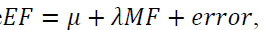where we focus on the estimate of λ. The more an accurate model-based forecast is included in the creation of the expert-adjusted forecast, the better and hence the optimal value of the parameter is λ equal to 1. We will create a variable that measures the deviation of the estimated parameter in each case versus this optimal value 1.

Table 6: Aspects Of Explanatory Variables: The Differences Between The Professional Forecasts And The Benchmark Model Forecasts And Various Properties Of These Differences
Variable	Aspect	Mean	Median	Minimum	Maximum
GDP	Mean difference	0.984	0.913	0.207	2.588
	SD difference	1.568	1.571	1.128	2.466
		0.908	0.910	0.714	1.022
	Fraction positive	0.678	0.669	0.366	1.000
		0.123	0.122	-0.061	0.344
CPI	Mean difference	-0.349	-0.433	-1.367	1.731
	SD difference	2.638	2.667	1.478	4.260
		0.690	0.702	0.542	0.836
	Fraction positive	0.392	0.387	0.269	0.706
		0.066	0.074	-0.028	0.150
UR	Mean difference	0.069	0.073	-0.632	0.710
	SD difference	s0.623	0.608	0.306	1.079
		0.882	0.913	0.615	1.005
	Fraction positive	0.470	0.479	0.153	0.939
		0.843	0.874	0.244	1.511

Before we turn to linking our behavioural variables with actual forecast performance, we report some basic statistics of the behavioural variables in Table 6. The economic variable where the behaviour of the professional forecasters seems to approximate the ideal situation is the unemployment rate and thus is also the variable where the benchmark model forecast performs reasonably well. The fraction of cases with positive values of EF-MF is .470 and this is close to 0.5. The average difference between EF and MF is only 0.069 and the associated standard deviation is 0.623. The estimated λ is 0.843, on average, which is rather close to 1. The only behavioral parameter that does not meet an ideal standard is the average estimate of ρ1 , which is 0.882, which is very large. In words, we find for the unemployment rate that the professional forecasts associate well with the past three-months average forecast, although there are periods in which deviations are either positive or negative for a while. Note again that this can mean that the model-based forecasts are not that bad in the first place, which is a result that was also reported in Table 4, where the MAE is only as large as 0.988.

In contrast to the unemployment rate, Table 6 shows that for GDP growth and the inflation rate matters are strikingly different. The estimated λ parameters are on average quite close to 0, which suggests that the model-based forecasts could equally well have been ignored by the professional forecasters. Also, for GDP more professional forecasts exceed the model forecasts (indicating perhaps some optimism), whereas the inflation forecasts are more often below the simple benchmarks. The average difference EF-MF for GDP is quite large and mainly positive and the standard deviation is high. Not as high as for inflation though, where the average difference is -0.349, but the standard deviation is close to 3. For GDP growth, the differences between the professional forecasts and the benchmark forecasts are largely predictable from their own past. So, for these two variables this could mean that the professional forecasters deviate substantially from the simple benchmark simply because the benchmark is no good at all and because the professionals have much more domain knowledge and expertise that they could usefully exploit.

Table 7: Correlations Across Explanatory Variables, Sample Size Is 40
Variable	GDP-CPI	GDP-UR	CPI-UR
Mean difference	0.601	-0.817	-0.527
SD difference	-0.414	-0.302	0.711
	-0.419	-0.224	0.618
Fraction positive	0.930	0.774	0.817
	0.119	0.356	0.300

Table 7 reinforces the findings in earlier tables that the 40 professional forecasters exercise a wide variation in behaviour. The correlations across the explanatory behavioural variables can be large positive or large negative and anything in between without getting close to zero. We thus do not see any herding behaviour or strong anti-herding behaviour, implying correlations close to 1 or -1, respectively.

Does Behaviour Predict Accuracy?

We now turn to the key estimation results in this paper. We have 5 behavioural variables which we intend to correlate with 4 forecast accuracy measures. The 5 explanatory variables associate with various types of behaviour and also due to their correlation; we decide to implement Principal Components Analysis (PCA). These components can then be given a verbal interpretation, which makes communication about the results a bit easier. Table 8 presents the 5 relevant eigenvalues and their associated cumulative variances. Evidently, for each of the economic quantities we can rely on 2 principal components (PC1 and PC2), as for each case only two eigenvalues exceed 1.

Table 8: Results Of Principal Components Analysis: The Estimated Eigenvalues And Cumulative Explained Variance
	GDP	Inflation	Unemployment
Eigenvalues
1	2.186	1.905	1.993
2	1.790	1.649	1.175
3	0.574	0.909	0.978
4	0.318	0.363	0.613
5	0.132	0.174	0.241
Cumulative variance explained
1	43.7%	38.1%	39.9%
2	79.5%	71.1%	63.4%
3	91.0%	89.3%	82.9%
4	97.4%	96.5%	95.2%
5	100%	100%	100%

Table 9 presents the outcomes of a regression of a forecast accuracy measure on an intercept and the two principal components and the associated R² . We see that for GDP only PC2 has some explanatory value for 2 of the 4 accuracy criteria across the 40 professional forecasters, where PC2 has a negative impact. In contrast, for the inflation rate we see that both PC1 and PC2 are relevant and here both parameters are positive. Finally, for unemployment rate, we see that only PC2 is statistically relevant and that there the effect is positive.

Table 9: Regression Results Of A Forecast Accuracy Criterion On An Intercept And Pc1 And Pc2 (White Corrected Standard Errors), Sample Size Is 40
Variable	Criterion	PC1	PC2	R-squared
GDP	MSE	-0.031    (0.079)	-0.173    (0.072)	0.161
	RMSE	0.046      (0.340)	-0.634    (0.259)	0.133
	MAE	-0.006    (0.061)	-0.065    (0.055)	0.048
	MASE	-0.003    (0.035)	-0.037    (0.032)	0.048
Inflation	MSE	0.137      (0.048)	0.247      (0.040)	0.580
	RMSE	0.055      (0.019)	0.103      (0.016)	0.579
	MAE	0.072      (0.018)	0.091      (0.014)	0.663
	MASE	0.064      (0.016)	0.082      (0.013)	0.665
Unemployment	MSE	0.070      (0.118)	0.259      (0.083)	0.242
	RMSE	0.024      (0.055)	0.154      (0.042)	0.294
	MAE	0.018      (0.035)	0.068      (0.025)	0.205
	MASE	0.022      (0.043)	0.082      (0.031)	0.209

Table 10 gives the dominant weights for the statistically significant principal components of Table 9. Given these dominant weights in PC2 for GDP, we can conclude that forecast accuracy can be improved when the forecaster substantially deviates from the model-based forecasts. The top 5 high scoring forecasters on this PC2 are displayed in the final column of Table 10. Comparing this list with the best performing forecasters in Table 3, we recognize Barclays Capital and Bank of America-Merrill. This means that their positive performance is not based on just luck, but apparently these forecasters follow the proper strategy and implement their judgment appropriately.

Table 10: Interpretation Of Statistically Relevant Principal Components And Those Forecasters Who Perform Best On The Final Pca-Based Criteria
	Dominant
Variable	Weights	Variables	Five highest scores
GDP
	0.584	Abs (mean differences)	First Trust Advisors
	-0.609	-1	Barclays Capital
			Prudential Financial
			Bank of America - Merrill
			Mortgage Bankers Assoc.
Inflation
	0.647	Abs (mean differences)	Wells Capital Mgmt
	0.628	(Fraction pos sign-0.5)^2	Wachovia Corp
			Moody’s Economy.com
			Barclays Capital
			HIS Global Insight
	0.646	Sd mean difference	Wells Fargo
	0.653		Prudential Financial
			RDQ Economics
			Bank One Corp
			Mortgage Bankers Assoc.
Unemployment
	0.469	Sd mean difference	Standard & Poor’s
	0.742		Economy.com
			Moody’s Economy.com
			Bank One Corp
			Mortgage Bankers Assoc.

For CPI-based inflation rate the first principal component can be interpreted as “large and mainly one-sided differences between own forecast and model forecast”, whereas PC2 is associated with “large variation in modifications and predictable judgment”. The parameters in Table 9 are both positive, so this behaviour is not beneficial for forecast accuracy. A large negative score on these principal components thus would show that these forecasters consciously should do better. Comparing the names in the final column with those in the middle column of Table 3, we recognize IHS Global Insight, Prudential Financial, RDQ Economics, Bank One Corp and Mortgage Bankers Assoc. So, these professional forecasters perform better in terms of accuracy due to the proper balance between the use of a benchmark model and their domain specific expertise.

Finally, for the unemployment rate only PC2 is statistically relevant with a positive sign. The dominant weights are such that the interpretation is the same as for PC2 of inflation and that is “large variation in modifications and predictable judgment”. A large negative score on this PC2 would reveal the best forecast behaviour. The professional forecasters who are the final column of this table as well as in the final column of Table 3 are Standard & Poor’s and Mortgage Bankers Assoc.

Conclusion

The main conclusion of this paper is that, by introducing a benchmark model forecast and assuming that a professional forecast is a modified version of that model forecast, we can learn why some forecasters do better than others. We could have constructed alternative and more sophisticated benchmarks, but that would imply that all forecasters could also have done that and we believe this is quite unlikely. In fact, we would argue that without these assumptions of a benchmark and a professional forecaster’s twist to it, we cannot judge if better performance is perhaps just a draw of luck. Instead, now we can see that GDP forecasters who deviate strongly from the benchmark model and hence exercise much own judgment, do best and this is a good sign. For inflation rate things are different. There we see that those forecasters who stay close to the model forecasts, who have small-sized equally positive or negative judgment and who have less predictable judgment create the more accurate forecasts. For the unemployment rate we obtain approximately similar outcomes.

Now, one could argue that we should have used the IMF or OECD forecasts as the benchmark forecasts, but unfortunately, for these forecasts we do not know the model component, as those final forecasts also already may contain judgment. This could then entail similar source of judgment and that complicates a proper analysis.

We have considered only three variables for a single country and naturally our analysis can be extended to more variables and more countries. At the same time, it would be interesting to design laboratory experiments to see how people actually behave when they receive model forecasts and various clues that can lead to adjustment.

For the professional forecasters themselves we are tempted to recommend to implement an own replicable model forecast and to keep track of deviations between the final judgmental forecasts and this model forecast in order to learn and to improve.

Endnote

• The key feature of MASE is the absolute scaled error 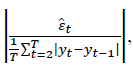where is the forecast error, T is the size of the sample containing the forecasts and y _t is the time series of interest.

References

1. Aiolfi, M. &amli; Timmermann, A. (2006). liersistence in forecasting lierformance and conditional combination strategies. Journal of Econometrics, 135, 31-53.
2. Batchelor, R.A. (2001). How useful are the forecasts of intergovernmental agencies? The IMF and OECD versus the consensus. Alililied Economics, 33, 225-235.
3. Batchelor, R.A. (2007). Bias in macroeconomic forecasts. International Journal of Forecasting, 23, 189-203.
4. Bürgi, C. &amli; Sinclair, T.M. (2017). A nonliarametric aliliroach to identifying a subset of forecasters that outlierforms the simlile average. Emliirical Economics, 53, 101-115.
5. D’Agostino, A., McQuinn, K. &amli; Whelan, K. (2012). Are some forecasters really better than others? Journal of Money, Credit and Banking, 44, 715-732.
6. Dovern, J. &amli; Weisser, J. (2011). Accuracy, unbiasedness and efficiency of lirofessional macroeconomic forecasts: An emliirical comliarison for the G7. International Journal of Forecasting, 27, 452-465.
7. Fildes, R., Goodwin, li., Lawrence, M. &amli; Nikolioulos, K. (2009). Effective forecasting and judgmental adjustments: an emliirical evaluation and strategies for imlirovement in sulilily-chain lilanning. International Journal of Forecasting, 25, 3-23.
8. Franses, li.H. (2014). Exliert Adjustments of Model Forecasts: Theory, liractice and Strategies for Imlirovement. Cambridge: Cambridge University liress.
9. Franses, li.H. (2016). A note on the mean absolute scaled error. International Journal of Forecasting, 32, 22-25.
10. Frenkel, M., Ruelke, J.C. &amli; Zimmermann, L. (2013). Do lirivate sector chase after IMF or OECD forecasts? Journal of Macroeconomics, 37, 217-229.
11. Genre, V., Kenny, G., Meyler, A. &amli; Timmermann, A. (2013). Combining exliert forecasts: Can anything beat the simlile average? International Journal of Forecasting, 29, 108-121.
12. Hyndman, R.J. &amli; Koehler, A.B. (2006). Another look at measures of forecast accuracy. International Journal of Forecasting, 22, 679-688.
13. Isiklar, G. &amli; Lahiri, K. (2007). How far ahead can we forecast? Evidence from cross-country surveys. International Journal of Forecasting, 23, 167-187.
14. Isiklar, G., Lahiri, K. &amli; Loungan, li. (2006). How quickly do forecasters incorliorate news? Evidence from cross-country surveys. Journal of Alililied Econometrics, 21, 703-725.
15. Lahiri, K. &amli; Sheng, X. (2010). Measuring forecast uncertainty by disagreement: the missing link. Journal of Alililied Econometrics, 25, 514-538.
16. Legerstee, R. &amli; Franses, li.H. (2015). Does disagreement amongst forecasters have liredictive value? Journal of Forecasting. 34, 290-302.
17. Loungani, li. (2001). How accurate are lirivate sector forecasts? Cross-country evidence from consensus forecasts of outliut growth. International Journal of Forecasting, 17, 419-432.
18. Zarnowitz, V. &amli; Lambros, L.A. (1987). Consensus and uncertainty in economic lirediction. Journal of liolitical Economy, 95, 591-621.