Research Article: 2017 Vol: 21 Issue: 3
Correlation, Association, Causation and Granger Causation in Accounting Research
Alireza Dorestani, North-eastern Illinois University
Sara Aliabadi, North-eastern Illinois University
Keywords
Correlation, Association, Causation, Granger Causality, Pairwise Granger Causality, Advanced Granger Causality, Regression.
Introduction and Prior Studies
In econometrics textbooks the most commonly used representation is a structural equation model (SEM). This form of econometrics representation is so important that almost all econometrics textbooks start with discussions of SEM. As an example, Stock and Watson (2011) examine the effect of excise cigarette taxes on the extent of smoking. They use the following model for their analysis:
Y = β X + ε
In this equation, the dependent variable, Y, is the extent of smoking, the independent variable, X, is the excise cigarette tax, and ε is the effects of all other variables that are not included in the model. The critical condition for using this model to estimate the β coefficient (called the effect coefficient) is that X and ε must be independent of each other. The independence of X from ε is known as the exogeneity of X or X being an exogenous variable. They argue that if all underlying assumptions of the SEM are maintained, then the model can answer all questions related to causal relationships.
Haavelmo (1944) concludes that in the linear equation of Y = β X + ε, the β X is the expected value of Y given that we set the value of X at x or simply set β x = E[Y?do(x)], which is different from the conditional expectation (Pearl, 1995). Chen and Pearl (2013) argue that the above interpretation has been misunderstood or questioned by many econometricians. For example, Goldberger (1992) agrees with the interpretation that considers β X to be the expected value of Y given that x is fixed, while Wermuth (1992) disagrees with Goldberger and argues that β X is not E[Y?x].
The main difference between Goldberger and Wermuth’s interpretations, in which econometrics textbooks fall, is whether the structural equations imply a causal meaning or not. Some econometrics textbooks posit that SEM equations represent causal relationships while other textbooks posit that the SEM equations represent the joint probability distribution. These two points of views are the extreme points and most econometrics textbooks fall somewhere between these two.
Chen and Pearl (2013) argue that the main source of confusion is the lack of precise mathematical definition of casual relationship. They state that SEM equations are used for two different purposes: one is for predictive problems and the other one is for causal problems or policy decisions. In predictive problems, one seeks to answer the question of what the value of Y will be given that we observe the value of X to be x. In predictive problems we can define β by the expression of β x = E[Y?do(x)], but it is incorrect to define β in the same way for casual relationship.
Another relevant concept is the concept of ceteris paribus. The concept of ceteris paribus that is widely used in economics is directly linked to causal relationship. In econometrics when we talk about definition of demand, we state that when the price of a good rises, then the quantity demanded will decrease ceteris paribus or holding other factors fixed. With the same notion when we hold all other variables fixed, or ceteris paribus, then any relationship between Y ad X, in Y = β X + ε relationship, must be a causal relationship.
Another concept that is tied to causal relationship is the discussion of X to be an exogenous variable. The exogeneity of X in a linear relationship between Y and X is held when X is independent of all other factors (variables) included in ε. For example, in a completely randomized process in which all participants are randomly assigned to either the control or treatment groups, independent of characteristics of the subjects, we can argue that X is exogenous. This interpretation of the exogeneity of X is different from the alternative interpretation in which we define β X as E[Y?X]. In other words, if the researcher is only interested in conditional expectation, prediction, then the causal relationship is of no importance. This argument is consistent with textbooks authored by Hill, Griffiths and Lim (2011).
As discussed earlier, the equation representing the relationship between Y and X, it is necessary for X to be exogenous. That is, the X must be independent of ε in order to estimate β in Y = β X+ε relationship. In this equation, ε is the effect of all other variables causing change in Y that are not included in X. The β represents the change in Y when X changes by one unit when we hold all other variables fixed, ceteris paribus. In addition, Chen and Pearl (2013) argue that if we incorrectly consider β X to be the expected value of Y given X or E[Y?X], then the statement of independence of X of ε will be meaningless. In this context, the E[Y?X], is called the conditional expectation of Y. If we are only interested in conditional expectation, then any bias in causal relationship can be ignored, and we can reliably use the regression equation for estimating α or the slope of the equation, E[Y?X] = α X in a linear relationship.
Furthermore, Chen and Pearl argue that if through randomization we force the exogeneity to X, then we will not estimate the conditional expectation but the interventional expectation. They added that conditional expectation and the interventional expectation are not the same. They posit that “by requiring that exogeneity to be a default assumption of the model, we limit its application to trivial and uninteresting problems, providing no motivation to tackle more realistic problems (Chen and Pearl, 2013)”.
In short, we argue that in accounting research, researchers need to differentiate between correlation, association, causation, and Granger causation. Correlation is a statistical measure of relationship between two variables disregarding the effects of other variables. Correlation measure ranges between -1 and +1 with -1 indicating a perfect negative correlation and +1 indicating a perfect positive correlation. No correlation is represented by zero correlation. In calculating correlation measure no effort is made to control the effects of other related variables.
While in calculating correlation coefficient no effort is made to control the effects of other related variables, in calculating the association measure the researcher examines the relationship between two variables while holding the effects of all other related variables fixed. In other words, the association is represented by β in the relationship between Y and X, which indicates the extent of change in Y when X changes, holding the effects of all other variables, ε, fixed (ceteris paribus).
In study of the causation or the cause-effect relationship between two variables, researchers are concerned about the effect of X on Y. In other words, in the presence of causal relationship we posit that X causes changes in Y. For causation or cause-effect relationship between X and Y (for X to cause Y) to hold, three conditions must be present: (1) X and Y must vary together, (2) X must occur before Y, and (3) no other variables must cause change in Y. That is, the researcher should show that when X does not change, then there will be no change in Y. We believe that the third condition is the most difficult one to be achieved. This difficulty is probably the main reason that in accounting literature the causation or cause-effect relationship are rarely used or used incorrectly.
The difficulty of achieving a causal relationship between two variables moved researchers toward a special form of causation called “Granger Causation”. Granger (1969) for the first time introduced a specific form of causation later became known as “the Granger Causality”. He posits that if a variable Granger causes another variable, then we can use the past values of the first variable to predict the value of the second variable beyond the effects of past values of the second variable.
The above discussions reveal that the strongest relationship between two variables is a causal relationship or a cause-effect relationship; however, when it is not possible to show a cause-effect relationship, then the next strongest relationship is the Granger causality relationship. Furthermore, most accounting researchers are interested to use a linear model to fit their data. Even though a linear model may be a good approximation to fit data, the use of linear model may not be appropriate in many cases, as we have shown below.
In short, accounting literature is full of studies that examine the relationship between two variables, but in most cases researchers do not properly differentiate between correlation, association, and causation, and in many cases the researchers use these completely different terminologies interchangeably. Given the above discussions, the main purpose of this study is to (1) provide an example to show how the use of a linear relationship can be misleading in some cases, and (2) show how accounting research can extend beyond reporting only correlation and association. In our study, by using practical examples we show how the Granger causality test which is based on time-series analyses can be incorporated into accounting research.
Background and Practical Examples
Correlation
In statistics two correlation coefficients are calculated. The first one is the Pearson correlation coefficient and the second one is the Spearman correlation coefficient. The Pearson coefficient or the Pearson Product-moment correlation coefficient is a measure of the linear relationship between two variables. The Pearson correlation coefficient ranges from -1 to +1, with -1 represents total negative linear relationship, +1 represents total positive linear relationship, and zero represents no correlation between two variables. The Pearson coefficient is used when two variables, Y and X, are interval or ratio data. The formula used to calculate the Pearson correlation coefficient is:
Where:
ρX,Y=Pearson correlation coefficient
Cov=Covariance
σX=the standard deviation of X
σY=the standard deviation of Y
Cov(X,Y) = E[(X-µX)(Y-µY)]
The Pearson coefficient was first introduced by Kari Pearson (1895) who got this idea from Francis Galton in 1880s.
The Spearman correlation coefficient or the Spearman’s Rank-order correlation is the nonparametric version of the Pearson linear correlation. The Spearman correlation coefficient measures the strength as well as the direction of relationship between two ranked variables. The Spearman coefficient is used when two variables are ordinal data. The formula for calculating the Spearman correlation coefficient is:
Where:
ρ=Spearman correlation coefficient
di=difference in paired orders
n=number of cases
As an example of the linear correlation coefficient, we have calculated the Pearson correlation coefficient between two variables, quarterly net income (X) and stock price (Y) of General motors from the first quarter of 1979 until the last quarter of 2016. The calculated Pearson liner correlation coefficients are shown in Table 1:
| Table 1 Pearson Correlation Matrix |
||
| Price (Y) | Net Income (X) | |
| Price (Y) | 1.00000 | -0.08658 |
| Net Income (X) | -0.08658 | 1.00000 |
The above table shows that the stock price and quarterly net income of General Motors move in opposite direction although the magnitude of change is too far from unity or total negative correlation. As we discussed earlier, in calculating correlation coefficient we ignore the effects of other related variables.
The calculated Spearman or ranked correlation coefficients are shown in Table 2:
| Table 2 Spearman Correlation Matrix |
||
| Price (Y) | Net Income (X) | |
| Price (Y) | 1.00000 | 0.25225 |
| Net Income (X) | 0.25225 | 1.00000 |
The above table shows that the stock price and quarterly net income of General Motors move in the same direction when we use the Spearman correlation coefficient.
Associations
In association analyses the researcher examines the relationship between two variables while holding the effects of other related variables unchanged (ceteris paribus). Association is generally represented by the following equation:
Y = β X + ε (1)
Where:
Y=the dependent variable
X=independent variable or variables
β=slope of the equation
ε=effects of all other variables that are not included in the equation
In the following we examine the linear association between stock price and quarterly net income of General Motors (GM) by holding the effects of variables such as total assets, liabilities, cash and short term investment and dividend fixed. That is, we are running the following linear regression model:
Price = β0 + β1 NI + β2ASSET + β3LIABIL + β4CASH + β5DVD (2)
Where:
Price: Stock Price of GM at the end of the period
NI: Net Income of GM for the period
ASSET: Total assets of GM at the end of the period
LIABIL: Total liabilities of GM at the end of the period
CASH: Total cash and short term investment at the end of the period
DVD: Dividend paid for the period
The results of running the below model are shown in Table 3.The above table shows that if we hold the effects of variables such as assets, liabilities, cash and short term investment, and dividend fixed, then there will be no association between stock price and quarterly net income of GM. The same results hold when we examine the association between stock price and liabilities or stock price and dividend. However, there is significant positive association between stock price and total assets, and stock price and cash and short term investment when we hold the effects of other related variables fixed. As we mentioned before, association is an improvement over simple correlation relationship.
| Table 3 Output of Linear Regression Model (2) Dependent Variable: Price |
||||
| Variable | Coefficient | Std. Error | t-Statistic | Prob. |
| Const. | 33.27471 | 2.913504 | 11.42086 | 0.0000 |
| NI | 3.91E-06 | 8.75E-05 | 0.044645 | 0.9645 |
| ASSET | 0.000160 | 4.49E-05 | 3.569371 | 0.0005 |
| LIABIL | -7.02E-05 | 4.46E-05 | -1.573200 | 0.1182 |
| CASH_STI | -0.000895 | 9.63E-05 | -9.294673 | 0.0000 |
| DVD | 0.001628 | 0.001968 | 0.827111 | 0.4098 |
| R-squared | 0.513012 | Mean dependent var | 38.92902 | |
| Adjusted R-squared | 0.493532 | S.D. dependent var | 15.92523 | |
| S.E. of regression | 11.33344 | Akaike info criterion | 7.738111 | |
| Sum squared resid | 16055.85 | Schwarz criterion | 7.869800 | |
| Log likelihood | -500.8463 | Hannan-Quinn criter. | 7.791622 | |
| F-statistic | 26.33593 | Durbin-Watson stat | 0.580953 | |
| Prob(F-statistic) | 0.000000 | |||
Nonlinear Model
Further analysis of the above linear regression reveals that the relationship between net income and stock price of GM is not linear, so to come up with a non-near model that better represents the relationship between these two variables, we have examined data and alternative models and come up with the following model using an Autoregressive Conditional Heteroskedasticity (ARCH) model. Our data are from the first quarter of 1979 to the last quarter of 2016.

Where:
yt=Price of GM stock at the end of quarter t
yt-1=Price of GM stock at the end of quarter t-1
yt-3=Price of GM stock at the end of quarter t-3
xt= Net income of GM during quarter t
xt-1=Net income of GM during quarter t-1
xt-2=Net income of GM during quarter t-2
xt-3=Net income of GM during quarter t-3
The results of running Model (3) are shown in Table 3:
| Table 3 Output of Non-Linear Model (3) Dependent Variable Is yt |
||||
| Variable | Coefficient | Std. Error | z-Statistic | Prob. |
| Const. | 2.546087 | 1.394663 | 1.825593 | 0.0679 |
| yt-1 | 0.758581 | 0.080714 | 9.398428 | 0.0000 |
| yt-3 | 0.166931 | 0.084206 | 1.982401 | 0.0474 |
| xt | 5.95E-05 | 2.48E-05 | 2.400805 | 0.0164 |
| xt-1 | 8.73E-05 | 2.39E-05 | 3.659156 | 0.0003 |
| xt-2 | 0.000121 | 2.87E-05 | 4.217008 | 0.0000 |
| xt-3 | 0.000146 | 3.26E-05 | 4.473418 | 0.0000 |
Results of variance equation as well as other statistics such as adjusted r-squared and model selection criteria are shown in Table 3.1:
| Table 3.1 Results of Variance Equation and Other Criteria of Running Non-Linear Model (3) |
||||
| C | 4.162009 | 3.129710 | 1.329839 | 0.1836 |
| RESID(-1)^2 | 0.253625 | 0.100411 | 2.525865 | 0.0115 |
| GARCH(-1) | 0.667588 | 0.134890 | 4.949123 | 0.0000 |
| R-squared | 0.801205 | Mean dependent var | 37.26751 | |
| Adjusted R-squared | 0.792805 | S.D. dependent var | 15.83317 | |
| S.E. of regression | 7.207045 | Akaike info criterion | 6.625644 | |
| Sum squared resid | 7375.694 | Schwarz criterion | 6.827251 | |
| Log likelihood | -483.6105 | Hannan-Quinn criter. | 6.707554 | |
| Durbin-Watson stat | 1.923084 | |||
Plots of calculated autocorrelation as well as partial autocorrelation of residuals and squared of residuals are shown in Figures 1 and 2, respectively:
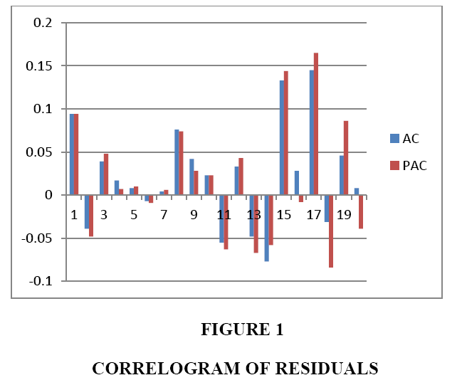
Figure 1: Correlogram of Residuals
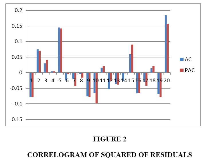
Figure 2: Correlogram of Squared of Residuals
The above figures show that there is no sign of autocorrelation or partial autocorrelation between residuals of estimated model, which indicate that the estimated model is reliable.
To show the robustness of our results using nonlinear model (ARCH), we have also conducted the Quandt-Andrew single break point test using a liner model. The results are calculated based on Hansen’s 1997 method are shown in Table 4. The null hypothesis of the Quandt-Amdrew test is no breakpoint within fifteen percent trimmed data. Our overall results reject the null hypothesis of no breakpoint. That is, the use of linear model is not appropriate for examining the relationship between stock price and net income of GM.
| Table 4 Quandt-Andrews Unknown Breakpoint Test |
||
| Statistics | Value | Prob. |
| Maximum LR F-statistic (Obs. 128) | 3.715142 | 0.0118 |
| Maximum Wald F-statistic (Obs. 128) | 26.00599 | 0.0118 |
| Exp LR F-statistic | 0.606979 | 0.4870 |
| Exp Wald F-statistic | 9.012185 | 0.0185 |
| Ave LR F-statistic | 1.006934 | 0.4276 |
| Ave Wald F-statistic | 7.048538 | 0.4276 |
| Note: probabilities calculated using Hansen's (1997) method | ||
The Bai-Perron test of multiple breakpoints test is also conducted and the results are shown in Table 5.
| Table 5 Bai-Perron Tests of Multiple Breakpoints Break test options: trimming 0.15, max. Breaks 5, sig. Level 0.05 |
|||||
| Sequential F-statistic determined breaks: | 5 | ||||
| Significant F-statistic largest breaks: | 5 | ||||
| UDmax determined breaks: | 3 | ||||
| WDmax determined breaks: | 4 | ||||
| Scaled | Weighted | Critical | |||
| Breaks | F-statistic | F-statistic | F-statistic | Value | |
| 1 * | 3.715142 | 26.00599 | 26.00599 | 21.87 | |
| 2 * | 4.164864 | 29.15405 | 33.59321 | 18.98 | |
| 3 * | 5.086327 | 35.60429 | 45.19244 | 17.23 | |
| 4 * | 4.703992 | 32.92795 | 46.31088 | 15.55 | |
| 5 * | 3.826573 | 26.78601 | 43.71717 | 13.40 | |
| UDMax statistic* | 35.60429 | UDMax critical value** | 22.04 | ||
| WDMax statistic* | 46.31088 | WDMax critical value** | 23.81 | ||
| * Significant at the 0.05 level. | |||||
| ** Bai-Perron (Econometric Journal, 2003) critical values | |||||
| Estimated break dates: | |||||
| 1: 128 | |||||
| 2: 74, 96 | |||||
| 3: 74, 96, 128 | |||||
| 4: 53, 75, 97, 128 | |||||
Consistent with the Qundt-Andrew single break point test, the Bai-Perron multiple break points test confirms the existence of multiple breakpoints, confirming that the use of nonlinear ARCH mode is preferable to a linear model.
To test for the stability of the coefficients, we have conducted the CUSUM test. The results are shown in Figure 3. Even though the diagram stays within the acceptable zone, it is clear that it approaches to the upper limit in one case. Figure 4 shows the behaviour of the residuals of our estimated ARCH model. Figure 5 shows the actual, fitted, and residuals of our estimated ARCH model. Lastly, Figure 6 shows the actual, fitted, and residuals if we incorrectly use a linear model to fit our data.
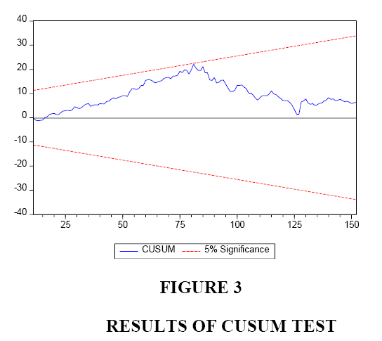
Figure 3: Results of Cusum Test
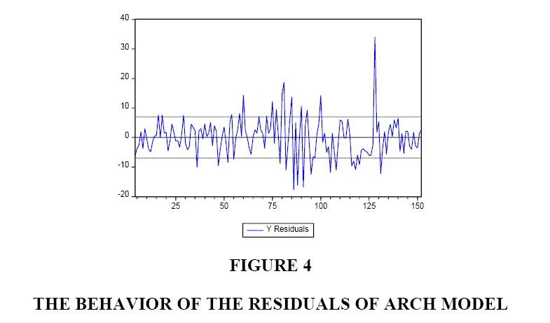
Figure 4: The Behavior of the Residuals of Arch Model
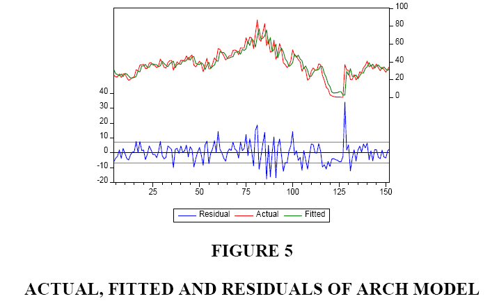
Figure 5: Actual, Fitted and Residuals of Arch Model
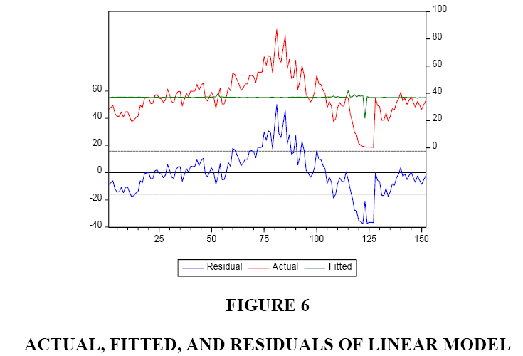
Figure 6: Actual, Fitted, and Residuals of Linear Model
All of the above tests results and figures confirm that the relationship between stock price (Y) and net income (X) of GM is non-linear and the use of a linear model is inappropriate.
Granger Causality
The results of the Pairwise Granger Causality test are shown in Table 6. The null hypothesis of this test is that one variable does not granger cause change in the other variable. As the results show, we cannot reject the null hypothesis that stock price (Y) does not Granger cause change in net income (X), but we reject the null hypothesis of net income (X) does not Granger cause change in stock price (Y). In other words, we conclude that the previous observations of quarterly net income of GM can help to predict stock price of GM, but previous stock prices do not help us to predict quarterly net income of GM.
| Table 6 Pairwise Granger Causality Tests |
|||
| Null Hypothesis: | Obs | F-Statistic | Prob. |
| X does not Granger Cause Y | 147 | 5.79765 | 7.E-05 |
| Y does not Granger Cause X | 0.55730 | 0.7325 | |
As we discussed earlier, the association reporting is an improvement over correlation reporting and Granger causality reporting is an improvement over the association reporting.
Policy, Practical and Educational Implications
Policy Implications
The discussions of differences between correlation, association, and the special case of causation (the Granger Causation) provided in this paper are of interest for regulators, standard setting bodies, and policy makers in evaluating the efficiency and effectiveness of new standards and rules. We posit that the causation can be used by regulators in evaluating the effects of their proposed regulations and standards. The causation and association can help investors to better evaluate the pattern of data and detect unusual changes in bottom line information.
Practical Implications
Correlation, association and special case of causation can be used in practice for different purposes such as detecting symptoms of fraud and irregularities. It is practical to use past data together with correlation or association analyses for forecasting future events. These forecasts can then be compared with actual data to detect unexpected fluctuations of data and investigate the differences between forecasted and actual data. These types of comparisons are of interests by both internal and external auditors. Both internal and external auditors, as part of their jobs, can develop hypotheses and then collect data to support or reject their hypotheses. Hypotheses are developed by evaluating the pattern of past data together with the use of correlation, association, or Granger causation.
Educational Implications
We believe that the accounting departments of different universities are not emphasizing enough on the differences between correlation, association, and causation, and in some situations students use these concepts inappropriately. Educating students about these important topics are of great importance for courses that deal with budgeting and forecasting. We posit that the inadequate understanding of correlation, association, and causation is the result of unfamiliarity of accounting students about these important topics. Therefore, we recommend that business schools incorporate these topics into their related courses and better educate students about these important topics.
Concluding Remarks
In this paper we discuss the differences between correlation, association, and Granger causation. We argue that these important topics are not used properly in accounting and auditing. In statistics two correlation coefficients are calculated. The first one is the Pearson correlation coefficient and the other one is the Spearman correlation coefficient. The Pearson coefficient or the Pearson Product-moment correlation coefficient is a measure of the linear relationship between two variables that are ratio data. The Spearman correlation coefficient or the Spearman’s Rank-order correlation is the nonparametric version of the Pearson linear correlation. The Spearman correlation coefficient measures the strength as well as the direction of relationship between two ranked variables. The Spearman coefficient is used when two variables are ordinal data. In correlation analysis, the focus is only on the change in the two variables and no effort is made to control the effects of other related variables. In association analyses the researcher examines the relationship between two variables while holding the effects of other related variables fixed (ceteris paribus).
In study of the causation or the cause-effect relationship between two variables, researchers are concerned about the effect of X on Y. For causation or cause-effect relationship between X and Y (for X to cause Y) to hold, three conditions must be present: (1) X and Y must vary together, (2) X must occur before Y and (3) no other variables must cause change in Y. The difficulty of achieving the third condition is probably the main reason that in accounting literature the causation or cause-effect terms are rarely used. The difficulty of achieving a causal relationship between two variables moved researchers toward a special case of causation called “the Granger Causation” that focuses on using the past values of the first variable to predict the value of the second variable beyond the effects of past values of the second variable.
We have provided practical examples for correlation, association, and the Granger causation and discuss their main differences. We have also showed, using an empirical example, how the use of a linear regression may not be appropriate when the true relationship is not linear. Finally, we have discussed the policy, practical and educational Implications of our paper.
References
- Chen, B. & Pearl, J. (2013) Regression and causation: A critical examination of six econometrics textbooks. Real-World Economics Review, 65, 2-20.
- Goldberger, A. (1992). Models of substance; comment on N. Wermuth, on block-recursive linear regression equations. Brazilian Journal of Probability and Statistics, 61(56).
- Granger, C.W.J. (1969). Investigating causal relations by econometric models and cross-spectral methods. Econometrica, 37(3), 424-438.
- Haavelmo, T. (1944). The probability approach in econometrics (1944). Supplement to Econometrica 12 12{17, 26{31, 33{39. Reprinted in D.F. Hendry & M.S. Morgan (Eds.), The Foundations of Econometric Analysis, Cambridge University Press, New York, 440(453), 1995.
- Hansen, B.E. (1997). Approximate asymptotic P-values for structural-change tests. Journal of Business and Economic Statistics, 15(1), 60-67.
- Hill, R., Griffiths, W. & Lim, G. (2011). Principles of Econometrics. (Fourth edition). John Wiley & Sons Inc., New York.
- Pearl, J. (1995). Causal diagrams for empirical research. Biometrika, 82(4), 669-688.
- Pearson, K. (1895). Notes on regression and inheritance in the case of two parents. Proceedings of the Royal Society of London, 58, 240-242.
- Stock, J. and Watson, M. (2011). Introduction to Econometrics. (Third edition). Addison-Wesley, New York.
- Wermuth, N. (1992). On block-recursive regression equations. Brazilian Journal of Probability and Statistics (with discussion), 61(56).