Keywords

GSTAR; SUR; Neural network; Cross covariance normalization.

Introduction

A neural network is perceived as a universal model as it does not require any statistical assumption (Zhang et al., 1998). This method is adapted from the neural system of the human brain (Hillary & Grafman, 2017; Khosravi et al., 2018; Li et al., 2018; Shanmuganathan 2016; Uddin et al., 2019; Vijh et al., 2020; Zhang et al., 2021). The neural network is a non-linear model that has been much developed until recently. Some researchers have proven that neural network is salient and potent to solve a number of problems in various disciplines (Zhang et al., 1998; Suhartono 2007). The neural network model has been frequently applied for non-linear time series. Some researchers applying neural network models for predicting time series are among others (Suhartono & Endharta 2011; Vlahogianni & Karlaftis 2013; Ostermark 1994).

One of the components of neural network model is input layer (He & Ma 2010; Henriquez & Kristjanpoller 2019; Prakash et al., 2011; Samani et al., 2007; Scholz et al., 2008; Yolcu et al, 2013). The input layer used in the neural network model is said to be more flexible, including the one on spatiotemporal data. Input layer could be in the forms of either raw or processed data resulting from the former model. Suhartono (2007) is the first paper using the input layer as that of time series in statistics. Since then, a lot more combinations between neural network and spatiotemporal models have come to be under investigation (Diani et al., 2013; Sulistyono et al., 2016).

This current research combined neural network and spatiotemporal methods. The research of Diani et al. (2013) merely made use of one neuron in the hidden layer. Sulistyono et al. (2016) chose to exclude the weight component from the input layer, though location weight is pivotal for the spatiotemporal model.

The renowned and developing spatiotemporal model is Generalized Space-Time Autoregressive (GSTAR), formerly introduced by (Ruchjana 2002; Iriany et al., 2013) further develop the GSTAR model into the GSTAR-SUR model. Location weight is an important component of the GSTAR model. Location weights that have been recurrently used are uniform location weight, distance inverse, and cross-correlation normalization (Suhartono & Atok, 2006; Suhartono & Subanar, 2006). The use of location weights does not only depend on the proximity of the location, but also on the characteristics of the data. There are some limitations in using uniform weights, distance inverse, and normalized cross-correlation. The weight of the location is not able to produce a model with good accuracy for rainfall data. The spatiotemporal model using cross-covariance normalized weights has better accuracy than using other location weights (Sulistyono et al., 2020; Sulistyono et al., 2019). This research was conducted to build a neural network model based on the normalized weights of the cross-covariance. Cross-covariance normalized weight of GSTAR-SUR model as input of neural network model on precipitation forecasting is an interesting topic in an area of developing importance. From the results of this study, it is hoped that a spatio-temporal model with a neural network approach will be formed which has a better accuracy rate than previous models and can be applied to forecast rainfall so that it is useful for farmers in determining the planting calendar.

Literature Review

Neural Network Model

Neural network (NN) is a time series method that attempts to imitate the learning process in the brain by using an artificial representation of the human brain (Aggarwal, 2018; Fitz & Romero, 2021; Marwala, 2013; Poulton, 2001; Ryland, 2021; Tymvios et al., 2008). This approach has been tweaked to mimic the way nerves in the brain function (Kusumadewi, 2010).

The architecture of the neural network model consists of three layers as shown in Figure 1, namely the input layer, hidden layer, and output layer. The input layer functions as a place where data is entered for further processing. The hidden layer is the processing unit of the data that has been entered. The output layer is where the output results from the process that has been carried out. While weights are weights that always change every time given input to the process.

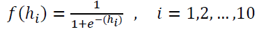
Important components in the model in neural network modeling are neurons, activation functions, and weights. Some of the activation functions include the activation function of binary, bipolar, linear, linear saturation, symmetric linear saturation, binary sigmoid, and bipolar sigmoid (Fausset, 1994). The activation function used in this study is a binary sigmoid logistic activation function, namely:

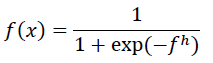
Where f ^h is a function in the hidden layer.

Back propagation is one of the algorithms used to update the weights on the neural network. In the back propagation algorithm, there is a forward phase and a backward phase. In the forward phase, the weights are calculated starting from the input unit to the output using a predetermined activation function. Then the error value is obtained which is the difference between the output value and the target value. While in the backward phase, the error is propagated backward from the output unit to the input unit, so that new weights are obtained that minimize the error (Siang, 2005).

In the back propagation algorithm, the resulting weight is influenced by the learning rate. The weakness in this algorithm is that the smaller the learning rate, the longer the learning process, on the other hand, if the learning rate is greater, the weight value will be far from the minimum weight (Apriliyah et al., 2008). Therefore, a new algorithm was developed, namely the resilient back propagation algorithm. The resilient back propagation algorithm uses the sign (positive or negative) of the gradient indicating the direction of the weight adjustment, while the size of the weight change is determined by the adjustment value (Riedmiller & Braun, 1992).

Normalized Cross-Covariance Weight

GSTAR model is formed by using cross covariance normalized weight. This sort of weight has been researched and applied by Apanasovich and Genton (2010) to predict pollution in California. The calculation of weight is as follow:

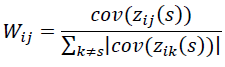(1)

The parameter is estimated by employing Seemingly Unrelated Regression (SUR) with the following formula.

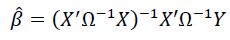(2)

Where is the variance-covariance matrix of GSTAR model residuals resulting from Ordinary Least Square (OLS) (Iriany et al., 2013).

In addition to the input layer, the other components of the neural network model are the hidden layer and output layer. One hidden layer was used and there were of maximum 10 neurons used in the hidden layer. The determination of the number of neurons used in the hidden layer was based on the lowest RMSE value. One neuron was used as the output layer (Suhartono, 2007). The output layer is represented in vector, of which component is location variable as in The used algorithm is the resilient backpropagation algorithm formerly used by (Apriliyah et al., 2008; Fadil et al., 2009) for estimating the sales of electricity load.

Data and Research Methodology

Data

The data, collected and analyzed in this current research, was in the form of 10-day precipitations during the period of 2005 to 2014. Those data were collected from the Meteorological, Climatological, and Geophysical Agency of Karangploso. The precipitation data were representing some locations where a majority of farmers reside in Malang Regency; the locations were in Junggo, Pujon, Tinjumoyo, and Ngujung.

Research Methodology

The research methodology used is design science research (DSR), where the design science research methodology is a methodology from the field of information systems that is useful for the development of new artifacts, such as service design construction, methods, and models (Teixeira et al., 2019).

The initial concept of this research was the determination of the input layer. The determination of which was focusing on the formation of the GSTAR-SUR model. It aimed at finding out significant variables of the model. The significant variables of GSTAR-SUR were then used as the input of the neural network model. Diani et al. (2013) assert that using significant variables on the GSTAR model as the inputs of neural network model yields more accurate forecasting than using all existent variables.

The steps of the data analysis process are as follows:

1. To test the stationarity of rainfall data on the variance and average. If the data is not stationary with respect to variance, a box-cox transformation is performed and if it is not stationary with respect to the mean, then differencing is performed.

2. Identify the real MPACF lag to determine the order to be used as the estimation of the GSTAR model.

3. Set the number of neurons in the input layer, hidden layer, and output layer.

4. The number of neurons in the hidden layer is based on the RMSE comparison, where the number of neurons in the hidden layer that produces the smallest RMSE is the number of neurons that will be used in NN modeling.

5. Determine the sigmoid activation function.

6. Determine the weights for each layer using the resilient backpropagation algorithm described in sub-chapter 2.5.

7. Calculation of cross-covariance normalized location weights.

8. Make CCF plots on rainfall data.

9. Estimating GSTAR-OLS parameters.

10. Calculate the matrix var (ε)=Ω.

11. Estimating GSTAR-SUR parameters.

12. Test the significance of the estimated value of the parameter. The estimated value of significant parameters will be entered into the GSTAR-SUR model.

13. Selection of the best model using the RMSE and R² criteria.

14. Forecasting rainfall data at each observation location.

Empirical Analysis

Data Identification

Precipitation is a vital factor for farmers in determining their planting patterns. Some locations in Malang Regency are mostly used as agricultural fields; they are Junggo, Pujon, Tinjumoyo, and Ngujung. The precipitations in the four locations were observed; there were in total 360 precipitation observations. The following stage of this research was forecasting the precipitations in those four locations. Each region has different precipitation intensity as shown in Table 1.

Table 1 Descriptive Statistics of Precipitations in Four Observed Locations
Location	Average	Standard Deviation	Minimum	Maximum
Junggo	6.248	6.954	0	35.800
Pujon	6.362	7.799	0	37.818
Tinjumoyo	4.948	5.683	0	29.000
Ngujung	5.012	5.902	0	35.600

The forecasting of precipitation was employing a neural network model by means of input as that in the GSTAR-SUR model. GSTAR-SUR modeling requires the data to be stationary against variance and average. The precipitation data were non-stationary against the variance, but they were stationary against average, and thus it required Box-Cox transformation, that is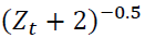 (Cryer & Chan, 2008). The stationary condition is to be fulfilled in order to find out significant parameters.

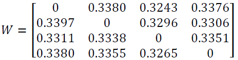
In the GSTAR-SUR model, there is the component of location weight. The location weight, in this current research, was cross-covariance weight. It was due to the relatively high variability of the precipitation data. This has been shown in Table 1 that the standard deviation value is higher than the average of each location. The location weight of cross-covariance normalization based on the stationary data is presented as follows:

The determination of time order in the GSTAR-SUR model is based on MPACF and MACF as shown in Figure 2. The spatial order used is 1. Figure 1 shows that the MPACF scheme cuts off up to lag 3; whereas the MACF scheme is shown to form a sine wave pattern. It means that the autoregressive order is said to be 3 and the moving average order is 0 (Wei, 2006). Therefore, the formed order of GSTARX-SUR is GSTARX-SUR (3₁).

NN-GSTAR-SUR Model

The formed neural network model was the one with the inputs of significant variables of GSTAR-SUR (3₁). This has been supported by research conducted by Diani et al. (2013) finding that the inputs of significant variables in the GSTAR-SUR model yield better forecasting than using all variables. Parameter forecasting was done by employing the SUR model as the GSTAR model constitutes a multivariate model. SUR method potentially solves inter residual correlation (Setiawan et al., 2016); accordingly, the parameter significance is more accurate compared to that in the Ordinary Least Square (OLS) method.

Parameter significance test on GSTAR-SUR model has resulted in 16 significant variables out of 24 variables. These 16 variables were treated as the input layer of the neural network model. The number of neurons in the hidden layer was limited to the range from 1 to 10 neurons and the best one was chosen based on RMSE value as shown in Table 2. The output layer had merely 1 neuron, in the form of a vector.

Table 2 RMSE Values in a Number of Neurons of Hidden Layer
The Number of Neuron in Hidden Layer	RMSE Value	The Number of Neuron in Hidden Layer	RMSE Value
1	0.1281	6	0.1227
2	0.1274	7	0.1207
3	0.1254	8	0.1172
4	0.1248	9	0.1178
5	0.1217	10	0.1162

The number of neurons used in the hidden layer was 10. It was due to the consideration that forecasting precipitation by means of 10 neurons in the hidden layer has yielded the lowest RMSE value, as shown in Table 2. Accordingly, the formed neural network model was NN (16, 10, 1) with the following architectural design.

Based on the architectural design in Figure 3, the equation of NN (16,10,1) - GSTAR-SUR (31) model is as below:

Where is the activation function of logistic sigmoid in the hidden unit which is defined as follow

(4)

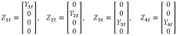
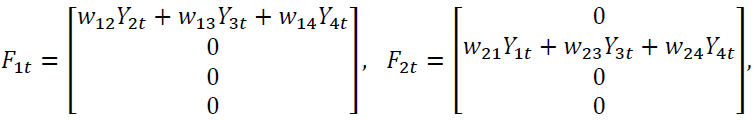
was formed from variables as those in GSTAR-SUR (31) model. It includes the lag of precipitation data in each location and the multiplication between cross-covariance location weight and the lag itself. The following formula presents some components of in lag 0.

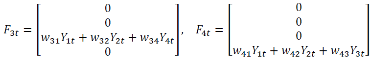
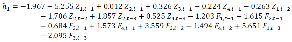
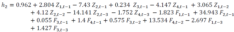
The followings are the neuron equations in the hidden layer.

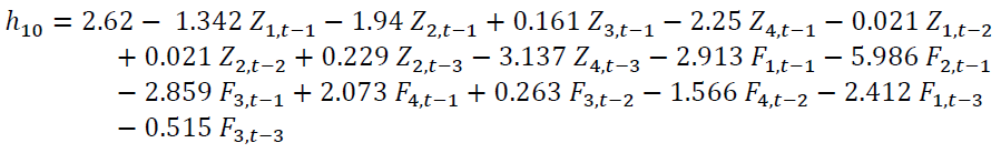
The reliability measurement of the NN (16,19,1) – GSTAR-SUR (31) model as shown in equation (3) was seen from RMSE and R² values. The following Table 3 displays RMSE and R² values for each location.

Table 3 RMSE and  R2 Values
Location	RMSE Value	R2 Value
Junggo	5.7830		0.5967
Pujon	5.8388		0.6412
Tinjumoyo	4.7784		0.5957
Ngujung	4.7486		0.6296
General	5.3131		0.6177

The results shown in Table 3 have imparted that NN (16,19,1) – GSTAR-SUR (31) model with cross-covariance normalized weight is proper and suitable for forecasting precipitations in Junggo, Pujon, Tinjumoyo, and Ngujung. It has been proven by the R² value of 61.77%. In Pujon, the R² value has reached 64.12%. Figure 4 presents the comparison between the actual values of precipitation and the precipitation forecasting results in Junggo, Pujon, Tinjumoyo, and Ngujung within 6 months, from July to December 2014.

Referring to Figure 4, the forecasting results by means of NN (16,19,1) – GSTAR-SUR (31) model with cross-covariance normalized weight have approached the actual data, though some dots are shown to be apart. However, the patterns resulting from this model are shown to resemble the actual data. It has been proven that NN (16,19,1) – GSTAR-SUR (31) model with cross-covariance normalized weight is reliable for forecasting precipitations in Junggo, Pujon, Tinjumoyo, and Ngujung.

Conclusion

A neural network constitutes a non-linear model requiring no statistical assumption. Along with the development of which, the neural network model has been frequently combined with time series and spatiotemporal models. This current research combined neural network and spatiotemporal models. One of the spatiotemporal models is the GSTAR-SUR model. The weight projected in this current research is cross-covariance normalized weight. This sort of weight is deemed suitable for data with high variability. The significant variable in the GSTAR-SUR model containing cross-covariance normalized weight was used as the input layer of the neural network model. The hidden layer made use of 10 neurons fulfilling the criteria of the lowest RMSE value and there was 1 neuron used as output. The data were in the form of 10-day precipitations in Junggo, Pujon, Tinjumoyo, and Ngujung, during the period of 2005 to 2014. The resulted model for forecasting precipitations in Junggo, Pujon, Tinjumoyo, and Ngujung is NN (16,19,1) – GSTAR-SUR (31). The cross-covariance normalized weight on the GSTAR-SUR model as input of the neural network model has yielded better forecasting. This model has been found to show the highest R² value, reaching 61.77%. Accordingly, this model is said to be reliable. To develop the current model and make it very useful for NN-GSTAR-SUR, the next research is included subset elements in the NN GSTAR-SUR model to improve forecast accuracy.

Academics and practitioners could use the model we used in our paper in many other areas, including, for example, exchange rate (Batai et al., 2017), agriculture (Moslehpour et al., 2018), tourism and transportation (Thipwong et al., 2020a,b; Tran et al., 2019). Readers may read Chang et al. (2017) for other areas that one could apply the model we used in our paper other areas. Extensions of our paper include applying the model used in our paper to analyze some important issues in other areas.

References

Aggarwal, C. C. (2018). Neural networks and deep learning. Springer.

Apriliyah, A., Mahmudy, WF, & Widodo, AW. (2008). Perkiraan Penjualan Beban Listrik Menggunakan Jaringan Syaraf Tiruan Resilent Backpropagation (RProp). Jurnal Ilmiah Kursor, 4(2).

Batai, A., Chu, A., Lv, Z., & Wong, W. K. (2018). China's impact on Mongolian exchange rate. Available at SSRN 3113165.

Chang, C. L., McAleer, M., & Wong, W. K. (2018). Management information, decision sciences, and financial economics: A connection (No. TI 2018-004/III). Tinbergen Institute Discussion Paper.

Cryer, J. D., & Chan, K. S. (2008). Time Series Analysis with Applications in R (2nd ed.). Iowa: Springer Science+Business Media, LLC.

Diani, K. A. N., Setiawan, & Suhartono. (2013). Pemodelan VAR-NN dan GSTAR-NN untuk Peramalan Curah Hujan di Kabupaten Malang. Jurnal Sains Dan Seni Pomits, 2(1), 19–24.

Fadil, J., Penangsang, O., & Soeprijanto, A. (2009). Load Forecasting for the Dstribution Network of South and Middle Kalimantan Using Artificial Neural Networks Resilient Propagation. Proceedings of National Seminar on Apllied Technology, Science, and Arts (1st APTECS). Surabaya.

Fausset, L. (1994). Fundamentals of Neural Network. New Jersey: Prentice Hall, Inc.

Fitz, S., & Romero, P. (2021). Neural Networks and Deep Learning: A Paradigm Shift in Information Processing, Machine Learning, and Artificial Intelligence. In The Palgrave Handbook of Technological Finance (pp. 589-654). Palgrave Macmillan, Cham.

He, F., & Ma, C. (2010). Modeling greenhouse air humidity by means of artificial neural network and principal component analysis. Computers and Electronics in Agriculture, 71, S19–S23.

Henriquez, J., & Kristjanpoller, W. (2019). A combined independent component analysis–neural network model for forecasting exchange rate variation. Applied Soft Computing, 83, 105654.

Hillary, F. G., & Grafman, J. H. (2017). Injured brains and adaptive networks: The benefits and costs of hyperconnectivity. Trends in Cognitive Sciences, 21(5), 385–401.

Iriany, A., Suhariningsih, Ruchjana, B. N., & Setiawan. (2013). Prediction of Precipitation Data at Batu Town Using the GSTAR ( 1 , p ) -SUR Model. Journal of Basic and Applied Scientific Research, 3(6), 860–865.

Khosravi, A., Koury, R., Machado, L., & Pabon, J. (2018). Prediction of wind speed and wind direction using artificial neural network, support vector regression and adaptive neuro-fuzzy inference system. Sustainable Energy Technologies and Assessments, 25, 146–160.

Kusumadewi, S. (2010). Membangun Jaringan Syaraf Tiruan Menggunakan Matlab & Excel Link. Tangerang: Graha Ilmu.

Li, Z., Li, J., Zhao, S., Yuan, Y., Kang, Y., & Chen, C. P. (2018). Adaptive neural control of a kinematically redundant exoskeleton robot using brain–machine interfaces. IEEE Transactions on Neural Networks and Learning Systems, 30(12), 3558–3571.

Marwala, T. (2013). Economic modeling using artificial intelligence methods. Springer.

Moslehpour, M., Bilgicli, I., Wong, W. K., Hua-Le, Q.-X. (2018). Meeting the Agricultural Logistics Requirements of Accommodation Enterprises in Sakarya, Turkey. Journal of Management Information and Decision Sciences 2 1(1).

Östermark, R. (1994). Using neural nets in modelling vector time series. Kybernetes.

Poulton, M. M. (Ed.). (2001). Computational neural networks for geophysical data processing. Elsevier.

Prakash, A., Kumar, U., Kumar, K., & Jain, V. (2011). A wavelet-based neural network model to predict ambient air pollutants’ concentration. Environmental Modeling & Assessment, 16(5), 503–517.

Riedmiller, M., & Braun, H. (1992). A Fast Adaptive Learning Algorithm. ProceedingS of the 1992 International Symposium on Computer and Information Sciences, 279–285. Antalya, Turkey.

Ruchjana, B. N. (2002). A Generalized Space Time Autoregressive Model and its Application to Oil Production Data. ITB.

Ryland, J. (2021). Modeling Axonal Plasticity in Artificial Neural Networks. Neural Processing Letters, 53(2), 1119–1146.

Samani, N., Gohari-Moghadam, M., & Safavi, A. (2007). A simple neural network model for the determination of aquifer parameters. Journal of Hydrology, 340(1–2), 1–11.

Scholz, M., Fraunholz, M., & Selbig, J. (2008). Nonlinear principal component analysis: Neural network models and applications. In Principal manifolds for data visualization and dimension reduction (pp. 44–67). Springer.

Setiawan, Suhartono, & Prastuti, M. (2016). S-GSTAR-SUR model for seasonal spatio temporal data forecasting. Malaysian Journal of Mathematical Sciences, 10, 53–65.

Shanmuganathan, S. (2016). Artificial neural network modelling: An introduction. In Artificial neural network modelling (pp. 1–14). Springer.

Siang, J. J. (2005). Jaringan Syaraf Tiruan dan Pemrogamannya Menggunakan Matlab. Yogyakarta: Andi.

Suhartono, & Atok, R. M. (2006). Pemilihan Bobot Lokasi yang Optimal pada Model GSTAR. Prosiding Konferensi Nasional Matematika XIII. Semarang.

Suhartono, & Endharta, A. J. (2011). Double Seasonal Recurrent Neural Networks for Forecasting Short Term Electricity Load Demand in Indonesia. Recurrent Neural Networks for Temporal Data Processing. doi: 10.5772/15062

Suhartono, & Subanar. (2006). The Optimal Determination of Space Weight in GSTAR Model by using Cross-correlation Inference. Journal of Quantitative Methods, 2(2), 45–53.

Suhartono. (2007). Feedforward Neural Networks Untuk Pemodelan Runtun Waktu. Universitas Gadjah Mada.

Sulistyono, A. D., Nugroho, W. H., & Iriany, A. (2019). Location Weight of GSTAR Model for High Variability of Rainfall Data. International Journal of Engineering & Technology, 8(1.9), 166–171.

Sulistyono, A. D., Nugroho, W. H., Fitriani, R., & Iriani, A. (2016). Hybrid Model GSTAR-SUR-NN For Precipitation Data. CAUCHY.

Sulistyono, A. D., Hartawati, H., Suryawardhani, N. W., Iriany, A., & Iriany, A. (2020). Cross-Covariance Weight of GSTAR-SUR Model for Rainfall Forecasting in Agricultural Areas. CAUCHY, 6(2).

Teixeira, J. G., Patrício, L., & Tuunanen, T. (2019). Advancing service design research with design science research. Journal of Service Management, 30(5), 577-592.

Thipwong, P., Wong, W. K., Huang, W. T. (2020a). Kano model analysis for five-star hotels in Chiang Mai, Thailand. Journal of Management Information and Decision Sciences, 23(1), 1-6.

Thipwong, P., Wong, W. K., Huang, W. T. (2020b). The impact comparison of supply chain relationship on public transportation quality in Taichung city, Taiwan and Chiang Mai city, Thailand. Journal of Management Information and Decision Sciences, 23(1), 16-34.

Tran, D. T., Moslehpour, M., Wong, W. K. Xuan, Q. L. H. L. 2019, Speculating Environmental Sustainability Strategy for Logistics Service Providers Based on DHL Experiences. Journal of Management Information and Decision Sciences, 22(4), 415-443.  

Tymvios, F. S., Michaelides, S. C., & Skouteli, C. S. (2008). Estimation of surface solar radiation with artificial neural networks. In Modeling solar radiation at the earth’s surface (pp. 221–256). Springer.

Uddin, L. Q., Yeo, B. T., & Spreng, R. N. (2019). Towards a universal taxonomy of macro-scale functional human brain networks. Brain Topography, 32(6), 926–942.

Vijh, S., Sharma, S., & Gaurav, P. (2020). Brain tumor segmentation using OTSU embedded adaptive particle swarm optimization method and convolutional neural network. In Data visualization and knowledge engineering (pp. 171–194). Springer.

Vlahogianni, E. I., & Karlaftis, M. G. (2013). Testing and Comparing Neural Network and Statistical Approaches for Predicting Transportation Time Series. Transportation Research Record: Journal of the Transportation Research Board, 2399(1), 9–22.

Wei, W. W. S. (2006). Time Series Analysis: Univarite and Multivariate (2nd ed.). USA: Pearson Education Inc.

Yolcu, U., Egrioglu, E., & Aladag, C. H. (2013). A new linear & nonlinear artificial neural network model for time series forecasting. Decision Support Systems, 54(3), 1340–1347.

Zhang, G. P., Patuwo, B. E., & Hu, M. Y. (1998). Forecasting with Artificial Neural Networks: The State of the Art. International Journal of Forecasting, 14.

Zhang, K., Robinson, N., Lee, S. W., & Guan, C. (2021). Adaptive transfer learning for EEG motor imagery classification with deep Convolutional Neural Network. Neural Networks, 136, 1–10.