Keywords

Budget Deficit, Economic Growth, Causality Test, VECM

Introduction

The Jordanian economy is one of the smallest economies in the Middle East. It suffers water shortage, and it is poor in oil and other resources which makes the government largely dependent on external aids from other countries around the world. In addition, the Jordanian government deals with other economic challenges that include high rates of unemployment and underemployment, budget deficit and deterioration in its current account. In addition, the government has large debts and loans.

Jordan suffers from a chronic deficit due to the fact that the revenue earned by the government is less than its expenditures. Since Jordan is a developing country with relatively limited economic resources, that deficit forms a huge economic burden on the country. A careful reading of the economic status of Jordan reflects clearly the hardships the government faces in financing the budget deficit. The government resorts to internal or external loans, which has largely increased the sum of loans in general since 2010. Furthermore, since the budget deficit forms a huge economic burden, and since it is very important for shaping the monetary and fiscal policy of the country, analyzing the budget deficit in Jordan in the period between 1990 and 2018, its development and determinants through time, and its impact on the economic growth is the target of this study.

The significance of the study rises through analyzing the deficit in the Jordanian budget, studying the factors that has led to its increase like Gross Domestic Product (GDP), economic structure, welfare state, and internal and external indebtedness, and evaluating the policies that the government follows in this field, and measuring the impact of this deficit on the economic growth. The researcher seeks to replenish the studies related to the determinants of the budget deficit in Jordan during the period between 1990 and 2018 and to analyze those determinants in order to avoid them in the future.

Ashour (2016) designed a flexible standard model using dynamic regression and cross-sectional data of 61 countries including Jordan for the years 2000–2013. That was for the goal of extracting the difficulties in financing the deficit of the Jordanian budget, specifically after 2010. Ashour also designed the model to avoid those difficulties in the future. The study designed a flexible criterion to measure the ratio of deficit in the budget in relevance to the Gross Domestic Product (GDP), and in comparison, with the used International Monetary Fund (IMF), which does not segregate countries according to their size, welfare, development, and structure. Furthermore, the study has designed a model that is able to give results with statistical values that are in line with the economic theory. Also, one of the most important recommendations the study has come up with that it was important for the government to focus more on the process of financing its budget deficit, especially after 2012 in which the government had faced a great hardship in financing its deficit domestically and internationally. Antwi (2013) analyzed the impact of the budget deficit in Ghana on its economic growth using time-series data from 1960 till 2010, and it used Granger causality test to analyze the relation between the expenditures and revenues of the government. The study resulted in the fact that the Ghanaian government continued to finance the piled deficit from the past without any consideration for the future budget. Risti & Nicolaescu (2013) studied the relation between the budget deficit in Romania and its economic growth. It resulted in finding the impact of the government’s expenditures on the commercial cycles on the long term, and it resulted in the fact that positive economic growth creates new revenues for the government. However, the government must avoid expanding its drawn fiscal policy as long as there is budget deficit and positive economic growth. Shahrour (2013) analyzed the economic impacts of the budget deficit in Syria. The study resulted in finding a direct correlation among the budget deficit, consumer spending, capital formation, and gross domestic product. On the other hand, there was not a statistically valuable correlation between the Syrian budget deficit and public saving but an inverse one between the budget deficit and unemployment. Paiko (2012) investigated the impact of financing the budget deficit in Nigeria, using econometrics methodology, because there has been a budget deficit since the independence of the country. The study found that financing the budget deficit led to inflation impacts and to a negative effect on investment spending. In addition, the study recommended focusing on the financial market in the process of financing the Nigerian budget deficit. Georgantopoulos & Tsamisa (2011) analyzed the impact of the budget deficit in Greece on the consumer prices index, exchange rates, and gross domestic product during the period between 1980 and 2009. The study resulted in finding one-direction causal connection among Greek budget deficit, consumer prices, and gross domestic product. However, it found no statistical value for the inflation variable in the used standard model.

Methodology and Data

This paper studies the determinants of the budget deficit and its impact on the economic growth using the descriptive approach, the analytical approach, and the econometrics methodology, the Granger Causality Test is used to determine the level of achievement of causal relationships between variables, and the Vector Error Correction Model (VECM) to examine the long run response of economic growth in Jordan to changes in Government budget deficit. This study analyzes data of the Jordanian general budget which the researcher has collected from the Jordanian central bank, as well as the financial reports generated from the ministry of finance.

Hypotheses

This study is based on the following hypotheses:

There is no impact that has a statistical significance at the rate of 5% for the budget deficit on the economic growth of Jordan.

Budget Deficit in Economic Literature

The following shows the schools that tackled the subject of “Budget Deficit” by analysis:

Classical Economics (The Classical School of Economics)

Classical economics is a school of economics that was first founded in Britain, in the late 18th and early-to-mid 19th century. The pioneers of this school are Adam Smith, Jean-Baptiste Say, David Ricardo, Thomas Robert Malthus, and John Stuart Mill. This school defends the free-market economy which arises clearly in Say’s law of markets. That law Supply creates demand that is equal to it, which means that the total supply must equal the total demand. In this case, there is no need for the government to interfere to reach market equilibrium, and that leads to an overall balance. Regarding the government’s revenues, specifically taxes, they are only used for covering the expenditures of the government. Moreover, the defenders of this school adopt the perception of keeping the government’s expenditures at its lowest, in order for the taxes not to increase, which lessens savings that would eventually impact investment and production. Classical economics also respects the sanctity of the government’s budget reaching equilibrium, and it considers budget deficit a vile sin that must be forbidden. Finally, classics economics lasted till 1929, when the Great Depression hit the economy of the United States of America and spread to the rest of the world. Then, it was unable to resolve that crisis.

Keynesian Economics (The Keynesian School of Economics)

Keynesian Economics is a school of economics founded by the British economist John Maynard Keynes. Its notions flourished in the post Great Depression era, when Keynes’ book, The General Theory of Employment Interest and Money was published in 1936. His book has started an intellectual revolution for economists. The book criticizes Say’s classic theory that supply creates equal demand. It also focuses on studying the economic behavior of individuals and companies (microeconomics) in order to study macroeconomics. In addition, the economy does not necessarily have to be at the point of full employment of the factors of production, and therefore Keynes was the first to indicate that the expansionary fiscal policy is capable of stimulating the economy and saving it from the bottom of the business cycle. Then, he suggested unbalancing the budget of the government by increasing its expenditures which can be financed by indebtedness and lessening taxes. That would shape a form of deficit in the budget that is capable of stimulating and increasing the total demand on the short term by increasing the consumer spending of families which incomes have increased. He believes that this would lead to stirring the economy cycle.

Neoclassical Economics

Milton Friedman is considered one of the most important thinkers of this school, whose ideas arose in the beginnings of the 80s of the previous century, when Keynesian economics proved unable to solve the crises of the market in the 70s. The crisis started when the focus on the government’s budget increased in most economies, and when the role of governments and interference in economy increased, which led to a rise in budget deficit of different countries. At the beginning, the subject of financing that deficit did not cause any fiscal problems, because the growth rate of the gross domestic product was higher than growth rate of the deficit. That lasted to the point in time, when the monetary system of Bretton Woods agreement collapsed. Then, the oil prices went up in 1973 and in 1979. Consequently, a new phenomenon called stagflation, persistent high inflation with high unemployment, emerged.

When arguments about the role of governments in the economic activity and budget deficit escalated among economists, neoclassicists came up with theories based on theories of classicists but with a new image. In those theories, neoclassicists hypothesized the rationality of consumers and efficiency of markets. Accordingly, the impact of chronic deficit lessens the accumulation of capital in a country, but a temporary budget deficit would slightly affect the lessening of savings which would lead to an increased interest. Therefore, neoclassicists adapt the notion of reducing the role of government in economy life and limiting it within the frame of the processes of economic adjustments for the sake of increasing the welfare of the members of society. This is exactly the notion that the International Monetary Fund (IMF) adapts and follows nowadays.

Determinants of Budget Deficit

The International Monetary Fund (IMF) defines total budget deficit as the concept that focuses on general revenues and expenditures, and it defines current deficit as increasing current expenditures according to the increase in revenues.

Readers in economic literature can clearly notice that there are several factors which lead to the increase of the government’s expenditures, such as different forms of military expenses, and to not keeping up with revenues to growth in expenditures for several reasons including, tax evasion, financial and administrative corruption, the incapability of collecting government’s funds from different agencies that are bound to repayments, the increase of total governmental demands with the reduction of domestic product and tending to exporting, which negatively affect trade equilibrium and the budget of the government. Lastly, one other factor is long-term loans that carry interests that lead to draining the country’s economic capabilities.

Governmental deficit can be categorized as a traditional one, which is shown in the variance in total governmental expenditures and revenues, except indebtedness. Many countries have used that measure to evaluate the performance of their followed fiscal policies. In addition, many countries have also used the measure of current deficit to measure the variance in governmental current revenues and expenditures. Nevertheless, it does not include capital ones like buying and selling assets considering that increasing the governmental expenditures on investment resources does not change the county’s net assets because new loans get replaced by new assets.

Moreover, there is operational deficit that countries use to measure inflation conditions under which the deficit is equal to the government and public sector’s demands for loans with the part of their use, the part that compensates holder of debt securities for inflation, subtracted from those demands. This becomes clear in the cases of countries that increased interest rates according to inflation rates in the total budget deficit. However, structural deficit excludes the temporary factors that affect the general budget; those factors are the deviation of interest rates from their value on the long-term, and the changes in process and incomes. It also excludes fiscal revenues gained from selling governmental assets because they represent exceptional revenues.

The important question which needs to be answered is: what are the main reasons leading to governmental budget deficit? The answer would be the huge difference between the growth rates of general expenditures from one perspective, and the growth rates of general revenues from another. That difference can be measured by estimating the correlation between the relative change in general revenues and the relative change in general expenditures. It is referred to as “the degree of sensitivity in general revenues changes to general expenditures changes.”

D= (dR/S)/ (Ds/R)

In which:

D is the coefficient of revenues sensitivity to change relatively to general expenditures.

dR is the change in general revenues.

dS is the change in general expenditures.

R is the total value of general revenues.

S is the total value of general expenditures.

The value of the coefficient D represents the existence of a gap between the government’s revenues and its expenditures. If there is a continuous decrease in the value of D, there will be an increase in the budget deficit and vice versa. Economic analysts of developing countries can notice a decrease in the value of D for those countries, which explains the continuous increase in the rates of the governments’ budget deficit and its transition to a structural one. Now, the study is going to show in details the structural and economic reasons for the budget deficit since they are of value for the subject.

Structural Reasons

1) The incapability of some governments of finding various revenues to cover their annual expenditures which makes budget deficit a main trait for those governments.

2) Trying to avoid paying taxes by any means necessary like tax loopholes, tax exemptions, paying taxes in low-taxes countries, and tax evasion.

3) The existence of high-income classes in society, and the injustice in distributing wealth among the members of society, which negatively affects the government’s financial status. Regardless the fact that high-income individuals are bound to pay higher taxes, they always try to evade paying them legally. Therefore, if society consists of a high rate of high-income individuals, they will not contribute to paying many taxes, but they will continue to depend on welfare privileges, which increase the burden on the government’s expenditures.

4) The relative inefficiency of the government in providing public services makes the value of the provided services less, which leads to spending more money by the government in order to provide what the members of society need.

5) The continuous competition among politicians to satisfy society members leads to high levels of governmental support which increases the expenditures of the government with time.

6) The increase in the rate of population growth adds more burdens on the government’s expenditures.

Economic Reasons

1) Wanger’s law. It represents a general universal law that shows a phenomenon of a continuous increase in the government’s expenditures, and that is due to successive economic, social, and scientific developments. That phenomenon was spotted and explained by the German economist, Adolf Wanger (1883). His theory can be summarized as the following: the government’s expenditures grow in higher rate than the gross domestic product and take the shape of an increasing function with time. Wagner was inspired by observing the increase in expenditures of the German and American governments.

2) Economic Recession. Many factors play a role in shaping economic recession because of the complexity of the economic life and the effect of each part of the economic equation on the other. One of the recession traits is unemployment that differs in rate from one country to another. It increases the rates of poverty in the society, and it has unpleasant impacts such as affiliating with terrorist organizations, expanding crimes and illegal trades, and black markets.

3) Inflation.Budget deficit causes a case of inflation in the countries that depend on printing money and increasing bank credit that is granted to the public sector, in order to adjust the budget deficit. That inflation causes prices to go up continuously which leads to deterioration of the purchasing capacity of the local currency.

4) Long-term governmental loans and their interests that governments of developing countries depend on to deal with budget deficit.

5) Military Expenses. It plays a big role in increasing the expenditures of the governments of developing countries especially the ones that face outer threats or the ones that suffer from political and security instability.

6) The expansion of the government administration, the financial and administrative corruption, and the deterioration of the governmental performance led to more expenditure.

The sources of financing budget deficit and its impacts:

There are 3 sources for financing budget deficit:

1) Inflationary Financing (New Money Notes): When the government finance its budget deficit by new money supply (printing money notes), it leads to increasing money demand which causes an increase in inflation with the existence of an increase in the government’s expenditures that is higher than revenue.

2) Financing by Issuing Sate Bonds (Treasury Bills): Financing budget deficit using internal loans decreases the deficit in the budget because of draining the purchasing capacity for the sake of paying interests. In addition, internal loans do not cause inflation because they are local loans that consume extra purchasing capacity. In addition, it does not increase the deficit in the upcoming years, because the government enters the capital market as a competitor for the private sector.

3) Financing by External loans: When the country finds refuge in external loans, the local interest rates go down which leads to incapability of calculating capital since cash is being pushed outside the country where interest rates are high.

By analyzing the previous variables where total economic variables mutually influence each other, we can say that those variables affect the exchange rates negatively. For example, from one perspective, we can say that increasing money supply reduces the purchasing capacity of the currency which leads to lessening its value. From another perspective, pushing foreign currency outside the country decreases the country’s reserve of it. Finally, the reduction of interest rates increases the demand on local currency to complete transactions, and it increases the demand on foreign currency as well for the sake of speculation.

From the previously mentioned facts, we can clearly see the relation created between the governmental budget deficit and the deficit of the balance of payments. Nonetheless, we need to differentiate between the government’s procurement of goods and its expenditures on goods and foreign services.

The Development of Budget Deficit in Jordan

Jordan has been suffering from budget deficit since its establishment due to its limited resources and the political conditions of the Middle East. Hence, the government has been depending on foreign aids to compensate for that deficit. Regardless, the budget deficit problem has not been resolved but kept on getting worse, which made the government seek internal and external loans for the sake of financing its projects. Afterwards, those external loans became a burden on the government and its budget.

Table (1) shows the changes in budget deficit and its ratio to gross domestic product (GDP). From the table, it can be noticed that after calculating external grants, the budget deficit has gone up from JOD 94.4 million in 1990 to about JOD 727.6 million in 2018, which is a compound annual growth rate of about 12%. From an analytical perspective, the development of budget deficit can be categorized into to two stages. The first stage was within the time interval (1990-1998,) which was the economic adjustment stage for treating the impact of the economic crisis in 1989 and the impacts of the second gulf war in 1990. The second stage was within the time interval (1999-2018,) in which Jordan adapted a five-year development plan (1999-2003,) an economic social transformation program (2002-2004), and two economic adjustment plans, one was for the time interval (1999-2006) and the second was the national economic adjustment program (2012-2015) which was organized by collaboration between the International Monetary Fund and the World Bank.

Moreover, Table (1) shows that the budget deficit has gone up from JOD 94.4 million in 1990 to JOD 327.3 million in 1998, which is a compound annual growth rate of about 7.15%. Most of the increase in the deficit occurred in 1997 and 1998 in which the deficit ratio to gross domestic product exceeded 5.175% and 5.84% respectively, and those were relatively high ratios in comparison with the ones of previous years which did not exceed 3%. Those high ratios were due to volatility in foreign aid. For the second interval, budget deficit has gone up from JOD 327.3 million in 1998 to JOD 727.6 million in 2018 with an annual growth rate of about 4%. The deficit has largely grown in 2009 and 2010 because of the global economic crisis and another growth during the years 2011-2013 which was the result of the Syrian crisis and Arab spring in which the deficit ratio to GDP was (5.615%-8.784%.) However, that deficit has started to decrease relatively since 2015 because of the adjustment plans that Jordan has been adapting.

Table 1 The Results of The Development of Budget Deficit
Year	GDP(Million JOD)	Deficit/	Budget Deficit Ratio to GDP%	Total of revenues and aid(Million JOD)	Ratio of Total of revenues and aid from GDP%	Total Expenditures(Million JOD)	Total Expenditures as a ratio from GDP%
1990	2521.4	-94.4	-3.744	938.2	37.21	1032.6	40.95
1991	2736.9	-147.8	-5.4	1117	40.81	1264.8	46.21
1992	3424.3	67.5	1.9712	1358.7	39.68	1291.2	37.71
1993	3735.2	69.5	1.8607	1406.1	37.64	1336.6	35.78
1994	4206.9	44.6	1.0602	1537.3	36.54	1492.7	35.48
1995	4597.9	15.2	0.3306	1620	35.23	1604.8	34.9
1996	4799.1	16.6	0.3459	1723.2	35.91	1706.6	35.56
1997	5090	-263.4	-5.175	1620.8	31.84	1884.2	37.02
1998	5604	-327.3	-5.84	1701.4	30.36	2028.7	36.2
1999	5769.4	-140.4	-2.434	1815.9	31.47	1956.3	33.91
2000	6069.7	-119.8	-1.974	1850.3	30.48	1970.1	32.46
2001	6478.4	-155.6	-2.402	1967.9	30.38	2123.5	32.78
2002	6842.9	-205.1	-2.997	2016.6	29.47	2221.7	32.47
2003	7320.8	-79	-1.079	2363.3	32.28	2442.3	33.36
2004	8254.7	-116.8	-1.415	2814.2	34.09	2931	35.51
2005	9108	-40.4	-0.444	3063.9	33.64	3104.3	34.08
2006	10933.2	-391.5	-3.581	3468.9	31.73	3860.4	35.31
2007	12539.6	-568.5	-4.534	3971.5	31.67	4540	36.21
2008	15885.5	-338.2	-2.129	5093.7	32.07	5431.9	34.19
2009	17178.8	-1509.2	-8.784	4521.3	26.32	6030.5	35.1
2010	18609.6	-1045.2	-5.615	4662.8	25.06	5,708.00	30.67
2011	20288.8	-1383	-6.817	5,413.90	26.68	6,796.60	33.5
2012	21689.6	-1824	-8.41	5,054.30	23.3	6,878.20	31.71
2013	23611.2	-1318	-5.582	5,758.90	24.39	7,077.10	29.97
2014	25437.1	-583.5	-2.294	7,267.60	28.57	7,851.10	30.86
2015	26,925.10	-925.9	-3.439	6,797.10	25.24	7,722.90	28.68
2016	27,829.60	-878.6	-3.157	7,069.60	25.4	7,948.20	28.56
2017	28,903.40	-747.9	-2.588	7,425.30	25.69	8,173.20	28.28
2018	29,984.20	-727.6	-2.427	7,839.60	26.15	8,567.30	28.57

Source: The Jordanian Central Bank, Data of 50 years, The Jordanian Central Bank, Amman.

In light of the general budget for the year 2018 and the main indicators of economic performance, the number of expenditures reached JOD 9 billion, of which JOD 7.9 billion are current expenditures, accounting for 88% of the amount of general expenditures and JOD 1.1 billion are capital ones, which represent 12% of expenditures. In addition, while capital expenditures increased by JOD 128 million or 12.4% for the year 2014, current expenditures in the same year recorded an increase of about JOD 445 million, which is a 6% increase from their actual level for the year 2017.

As for local revenues and foreign grants for the year 2018, they were estimated at JOD 8.5 billion compared to JOD 7.7 billion for the year 2017 with an increase of about JOD 800 million or 10%. Also, foreign grants in 2018 resulted in a budget deficit of about JOD 543 million or 1.8% of Gross Domestic Product (GDP) compared to 2.6% of GDP in 2017.

Moreover, tax revenues represent about 65% of the total local revenues for the 2018. Those tax revenues consist of 13.9% of income and profit taxes, 2% of financial transactions taxes, 45.1% of goods and services taxes, and 4.6% of trade taxes. From another perspective, non-tax revenues constitute 34% of total revenues and they consist of goods and services sales revenues, revenues of property income, and other various revenues like mining, loan installments, and customs revenues of customs tax exempted goods.

Estimation and Results

The relationship between economic growth and the Government budget deficit will be analyzed through the following models:

GRi=β0+β1Di+ei (1)

Where:

GR: Percentage Change in Gross Domestic Product

D: Deficit/Surplus Including Grants

e: Error

Before beginning with data analysis, the stability of time series and whether they are static or not must be confirmed to avoid the problem of fake regression, which gives a high value for the interpretation coefficient and the time series stability test. For the study variables, the (Dickey- Fuller) test will be used. The test relies on an estimation of the following model:

yt= ρyt-1+ υt; ρ€ (-1, 1) (2)

When the first difference of both sides of the equation is taken, we obtain the following form:

yt - yt-1=ρyt-1 - yt-1+υt (3)

δ=ρ -1 (4)

yt=δ yt-1+Δ υt (5)

The null hypothesis shall be confirmed leading to confirming the presence of the unit root and, therefore, the nonstationary series against the alternative hypothesis which asserts the stationary series H0: δ ≥ 0 vs. H1: δ<0

Table 2 Augmented Dickey-Fuller Test
Variable	ADF		Level	First difference
	Critical values 1%	Critical values %5	ADF	ADF
D	-3.7	-2.97	-1.78	-6.8
GR	-3.7	-2.97	-2.2	-11.1

It is clear from Table (2) that the variables are nonstationary at a level and that they are all stationary at the first difference if the calculated value (absolute) is larger than Critical value. They, therefore, have similar integration degrees I (1) and cointegration between them can be tested.

The “Johansen Test” is used to test combined integration to identify the achievement of a relationship in the long run between the variables which are integrated at the same level. The Augmented Dickey Fuller Test is used for the unit root. It tests the level of presence of integrated equations in a combined manner for the directions of the study variables through determining the root significance distinguishing directions. The numbers of distinguished roots that are not zero express the matrix rank and are equal to the number of directions of independent combined integration. The presence of combined integration between them at the same level expresses a long-term stable relationship.

Table 3 Unrestricted Cointegration Rank Test (Trace)
Hypothesized No. of CE(s)	Eigenvalue	Trace Statistic	0.1 Critical Value	Prob.**
None *	0.382626	14.75303	13.42878	0.0645
At most 1	0.102230	2.696040	2.705545	0.1006

Table (3) shows the presence of one integration relationship between the study variables in Jordan. This indicates the presence of a causal effect from one or two directions between the study variables leading to the significance of dealing with the test that follows it according to the study plan to analyze this relationship. This shall be carried out through the Granger Causality Test. This test is used to determine the level of achievement of causal relationships between variables. To test the level of achievement of causal relationships between variables, the following formula shall be used:

It can be understood from the equation that time delay in the time series can lead to the creation of a predictive power between the study’s variables (Granger & Engle, 1987). The Causality Test indicates that the Government budget deficit has no effect on economic growth as the probability value reached (0.47). This is a statistically insignificant value. The Causality Test also indicates the presence of a positive effect by economic growth on the Government budget deficit as the probability value reached (0.93) (Table 4).

Table 4 Granger Causality Test
Null Hypothesis:	Obs	F-Statistic	Prob.
DIFICIT does not Granger Cause G	27	0.39735	0.5344
G does not Granger Cause DIFICIT		3.62942	0.0688

Using analysis of variance tool to identify the amount of variation in the prediction of each variable in the model. the Vector Error Correction Model (VECM) depends on following equations:

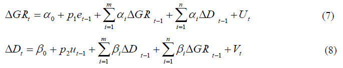
Our model contains cointegration relationship among the variables, then we can proceed to VECM (Table 5).

Table 5 Vector Error Correction Estimates
Cointegrating Eq:	CointEq1
GR(-1)	1.000000
DEFICIT(-1)	6.60E-06
	(3.8E-05)
	[ 0.17511]
C	-0.093195
Error Correction:	D(GR)	D(DEFICIT)
CointEq1	-0.409422	-2252.149
	(0.20595)	(1396.85)
	[-1.98794]	[-1.61231]
D(GR(-1))	-0.358204	-25.84061
	(0.18743)	(1271.20)
	[-1.91116]	[-0.02033]
D(DEFICIT(-1))	7.92E-06	-0.266233
	(3.0E-05)	(0.20335)
	[ 0.26412]	[-1.30925]
C	-0.008685	-36.77224
	(0.00954)	(64.7247)
	[-0.91007]	[-0.56813]
R-squared	0.500204	0.244300
Adj. R-squared	0.432050	0.141250
Sum sq. resids	0.051867	2385877.
S.E. equation	0.048555	329.3159
F-statistic	7.339312	2.370695
Log likelihood	43.93090	-185.4432
Akaike AIC	-3.071608	14.57255
Schwarz SC	-2.878055	14.76610
Mean dependent	-0.008222	-30.58077
S.D. dependent	0.064428	355.3688
Determinant resid covariance (dof adj.)		252.3826
Determinant resid covariance		180.6999
Log likelihood		-141.3437
Akaike information criterion		11.64182
Schwarz criterion		12.12571

The results showed the error term in economic growth equation was not significant, this means that economic growth in Jordan in the longer-term does not response to changes in Government budget deficit.

Conclusion and Discussion

In this study we investigate the relationship between economic growth and the Government budget deficit in Jordan, the Granger Causality Test indicates that the Government budget deficit has no effect on economic growth as the probability value reached (0.47). This is a statistically insignificant value. The Causality Test also indicates the presence of a positive effect by economic growth on the Government budget deficit as the probability value reached (0.93), and by using Vector Error Correction Model (VECM), The results showed the error term in economic growth equation was not significant, this means that economic growth in Jordan in the longer-term does not response to changes in Government budget deficit.

Therefore, this study recommends that when the government develops solutions to reduce the budget deficit, the proposed solutions should not affect the government's social responsibility towards the poor and low-income classes, especially low pension salaries, which are below the minimum, to achieve good life.

References

1. Abd, R., & Nur, H. (2012). The relationship between budget deficit and economic growth from Malaysia's perspective: An ARDL approach, IACSIT press. Proceedings from International conference on Economics, IPEDR, Singapore, 38.
2. Antwi, S. (2013). Consequential effect of budget deficit on economic growth: Empirical evidence from Ghana, Canadian Center of Science and Education. International Journal of Economics and Finance, 5(3).
3. Ashour, S. (2016). Determinants and financing the budget deficit: An analytical study on Jordan (1996-2014). PhD thesis, University of Jordan, Amman, Jordan.
4. Georgantopoulos, A., & Tsamism, A. (2011). The macroeconomic effects of budget deficits in Greece: A VAR-VECM approach. International Research Journal of Finance and Economics, 79.
5. Granger, C.W.J. (1969). Investigating causal relationship by econometric models and cross spectral methods. The Econometric Society, 37, 424-438.
6. Gujarat, D., & Porter, D. (2009). Basic econometrics, Print book, (5^th Edition). McGraw-Hill Irwin, Boston.
7. Khan, A. & Bartley, H.W. (2002). Budget theory in the public sector, (1^st edition). London and Connecticut: Westport.
8. Manasse, P. (2007). Deficit limits and fiscal rules for dummies. International Monetary Fund (IMF Staff Papers), 54 (3).
9. Milo, P. (2012). The impact of budget deficit on currency and inflation in the transition economies Sciendo, Poland. Journal of central Banking Theory and Practice, 1, 25-27.
10. Paiko, I. (2012). Deficit financing and its implication on private sector investment: The Nigerian experience, Oman. Arabian Journal of Business, and management, 1, 10.
11. Risti, L.C. (2013). Budget deficits effects on economic growth, University of Arad, Romania. Journal of Economics and Business Research, 1, 162-170.
12. Shahrour, I. (2013). The public budget deficit in Syria and its economic effects, Damascus University, Syria. Arab Economic Research, 63-64.