Research Article: 2021 Vol: 27 Issue: 5S
Disclosure of Confidential Financial Information Committed By Management and Its Impact on Stock Returns
Doaa Noman Mohammed Al Husseini, University of Mosul
Laila Adbulkarem Mohammed ALhashmi, University of Mosul
Keywords
Return, Transaction Volume, VAR Analysis
Abstract
Research focused on the divulgation principle, on the transparency of information and on an equal basis between all market dealers, be they shareholders, investors or the public, and its aim was to explain the signal and its meaning, and its features, the confidential or banned information contained in the Iraqi banking environment. This may result in a lack of faith between investors, shareholders and the public between investors, equities and the public. The most significant research leads to recommendations including the drafting of frequent reports on the degree of adherence with internal policy and methodologies for confidentiality and the promotion of employee culture and awareness. The aim of this study is to show that the trade volume and ISX return are dynamic (Iraq Stock Exchange). The daily performance of the ISX and the daily trading volume details was analyzed for this reason between 22.03.1993 and 22.03.2019. The research has developed a long-term relationship between volume and return, and a single-way causality has been achieved between volume and return. In the analysis used to more detail the relationship between the sequence, impulses and techniques for variance decomposition were studied and the shift in index price was concluded to be efficient for the transaction volume.
Introduction
The relationship between stock returns and transaction volume is one of the most studied topics in finance literature. Trading volume and stock prices are two important financial indicators that show the success of stock markets. Transaction volume affects the prices of financial assets as new information enters the market and also reflects changes in investors' expectations. Many studies have found that high stock market volume is associated with volatility returns.
There are some reasons that make the relationship between stock price and transaction volume important. First; the price-transaction volume relationship shows the structure of financial markets. The second is important for studies using transaction volume and price data. Another allows discussion on the empirical distribution of speculative price changes and provides important implications for futures market research (Hamad, & Ajesh 2021).
In one of the first studies on the price-volume relationship; Granger and Morgenstern (1963) could not find a relationship between different index returns and transaction volume in different periods in the USA between 1915 and 1961. Epps & Epps (1976) examined the relationship between stock price changes and trading volume and found a positive causality from trading volume to absolute stock returns. Rogalski (1978) found a positive relationship between monthly price changes and volume. Later, many studies were conducted to determine the existence and direction of the price-volume relationship for the markets of both developed and developing countries. In this study, a general literature study on the relationship between price changes in stock markets and transaction volume will be given, and the relationship between price and volume will be explained. In the application part of the study, the results are interpreted by including the data and the econometric model used.
Literature Review
Tauchen & Pitts (1983) modelled the change in prices and the co-distribution of transaction volume as a mixture of bivariate distributions. In their studies, they found a positive relationship between price changes and volume by using daily data in the United States.
Ali, (2006); Barik, Patra, Patro, Mohanty & Hamad (2021) using weekly data of the stocks of 29 companies traded on the ISX, found a co-integrated relationship between the stock price and transaction volume between January 8, 1988 and March 29, 1991.
Abdulla, (1995) examined the stock price-volume relationship in the stock markets of Latin American countries (Argentina, Brazil, Chile, Colombia, Mexico and Venezuela). Using monthly returns between January.1986 and April.1985, it was revealed that the volume affected price changes strongly and positively. At the same time, they found that transaction volume in Latin American markets affects stock returns, but stock returns do not affect volume.
Asaad (2014) using daily and weekly data between 1963-1996 in the USA, found that high volume portfolios affect the returns of low volume portfolios. They stated that the reason for this was that investors with a low volume portfolio react more slowly to the information entering the market.
Abu-Nassar (1996) found a positive and simultaneous relationship between return and volume of stocks outside of India in the stock markets of Latin American and Asian countries, as well as a two-way causality between return and volume.
Al-Mahmoud (2000) analyzed the dynamic relationship between stock returns and transaction volume in 9 major stock markets (USA, Japan, England, France, Canada, Italy, Switzerland, the Netherlands and Hong Kong) using daily data, using the EGARCH method between 1973-2000. In their studies, they found a significant and positive relationship between stocks and their returns and transaction volume. They also found that price changes were the cause of volume changes.
Kaehler (2014) emerging markets Toda-Yamamoto Granger used their weekly price and trading volume data using the method of causality.
Keef (2007) analyzed the daily data in Australian stock market between April 24, 1989 and December 31, 1993 with the GARCH method and reached findings that support the asymmetric relationship between price and volume. In the GARCH analysis, they found that the variance decreased when the transaction volume was taken as an exogenous variable according to the conditional variance. In the study, it was determined that the volume-price change slopes calculated for negative returns are smaller than positive returns. While this result shows the asymmetric relationship, this situation; it can be explained that negative price changes are more sensitive to transaction volume than positive price movements.
The study (Tripathy 2011), by means of bidirectional regression, VECM, VAR, IRF and Johansen co-integration tests, analyzed a relation between stock returns and transaction volumes in the Indian stock market. In his study, he stressed that the volume of transactions is related to the growth in return volatility, which is asymmetrical. This correlation illustrates the important effect of new knowledge on price volatility on the market every day. Another reason: investors are more reluctant to take downside risks. Investors are thus responding to negative news quicker. At the same time, a long-term causal association between stock return and transaction volume is determined by Tripathy (2011).
(Hahn, et al. 2013) analyzed the relationship between volatility of stock returns and trading volume in Korean stock market using daily data and GJR GARCH and EGARCH methods between January 2000 and December 2010. As a result of the analysis, they found a positive relationship between transaction volume and volatility. They stated that the transaction volume affects the information flow to the market and that the transaction volume also explains the volatility asymmetry.
Data and Methodology
In this study, the relationship between the return of the ISX 100 Index and the trading volume in the period 22.03.1993 and 22.03.2019 is analyzed. For this purpose, 6602 observations were obtained from the Central Bank Electronic Data Distribution System. Logarithmic returns of the ISX 100 Index are calculated by using the daily closing prices with the formula below. The transaction volume is also included in the analysis by taking its natural logarithm.

Unit Root Tests
In time series analysis, before detecting the existence of any relationship between series, their stationaries should be tested. For this purpose, Phillips–Perron test (PP) [15], Kwiatkowski-Phillips-Schmidt-Shin (KPSS) and Elliot et al. (1996) [9] Dickey Fuller Generalized Least Squares (DF-GLS) (ERS) (Dickey Fuller Generalized Least Square) tests were applied.
According unit root test, while null hypothesis series are not stationary (there is unit root); the alternative hypothesis is that the series are stationary (no unit root). The corresponding equation is as follows:
Equation---1
The LM-statistic value examined in the KPSS test should be compared with the critical values at 1%, 5% and 10% significance levels. If the LM-statistic value is large, it is concluded that the series is not stationary by rejecting the null hypothesis. The hypothesis of the KPSS unit root test is that the time series is stationary. The alternative hypothesis is that the time series is not stationary. The relevant equations are as follows:
Equation ---2

Equation ----3
Where t =1, 2, 3...T
Also in the study, recently, Elliot et al [9]. The DF-GLS (ERS) test developed by (1996) was applied. The DF-GLS (ERS) test is based on the process of de-trending the series, while the null hypothesis is that the series is not stationary (there is unit root); The alternative hypothesis is that the series are stationary (no unit root). The DF-GLS (ERS) test is estimated as follows:
Equation -----4
Return by Transaction Volume
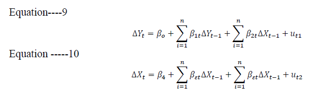
In this study, based on Tripathy (2011), multivariate models between index return and transaction volume are tested. These models can be shown as follows:
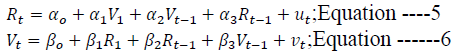
In the equations, Rt is the return; Vt is the transaction volume; α and β coefficients; u and v show the error terms. As can be understood from the above models, the return equation; It consists of the transaction volume, the transaction volume of the previous period and the return value of the previous period. Likewise, the transaction volume equation consists of the return, the return for the previous period and the transaction volume values for the previous period.
Johansen Cointegration Test
In this study, Johansen cointegration test was applied to determine the long-term relationship between series. The VAR model, which is the beginning of the Johansen Cointegration test, can be shown as follows:
Var Analysis
In the study, VAR Analysis was used to determine the relationship between transaction volume and yield. The reason for this is that the relationships in the model can be predicted in multiple ways. For this purpose, in the bivariate VAR equation, every variable is affected by its current and past values. Equations can be represented as follows:
Choosing the appropriate lag length is important in determining the VAR model. If the lag length is determined to be a shorter period than it should be, the coefficients lose their statistical significance. If the delay is taken larger than the required length, the variance values are high. In order to establish a correct and reliable model, it is important to determine the lag numbers of the variables. In the study, the Sequential Modified LR Test Statistic (LR), Final Prediction Error (FPE), Akaike (AIC) and Hannan-Quinn (HQ) information criteria were used to determine the length of the delay.
VAR Analysis is divided into basic sections: Granger causality, impulse response analysis and variance decomposition. Granger causality tests are intended to support the results found with the other two analysis tools. In Granger causality test, causality relationship between variables is sought. In variance decomposition, it shows what percentage of the change in the variance of each variable is explained by its own delay and what percentage is explained by the other variables. Impact-response analysis, on the other hand, is observed when one unit of shock is applied to one of the variables, the responses of both itself and other variables to this change. In this way, dynamic relationships between variables are observed.
Analysis and Findings
Unit Root Results
Table 1 and Table 2 show the stationarity results for the specified unit root tests. According to the unit root test results, it is revealed that the yield and transaction volume series are stationary and do not contain unit roots.
| Table 1 ADF, PP and KPSS Unit Root Tests (Level = I (0)) |
||||||
|---|---|---|---|---|---|---|
| PP Tests | KPSS Tests (LM) | DF-GLS Test | ||||
| Variables | Fixed | Fixed and Trended | Fixed | Fixed and Trended | Fixed | Fixed and Trended |
| Return | -69.8166*** | -69.8337*** | 0.4330** | 0.6610*** | -7.9463*** | -8.7811*** |
| Transaction Volume | -7.0444*** | -14.4941*** | 5.1141 | 1.5065 | -0.4483 | -1.7663 |
| Table 2 ADF, PP and KPSS Unit Root Tests (Level = I (1)) |
|||||||
|---|---|---|---|---|---|---|---|
| PP Tests | KPSS Tests (LM) | DF-GLS Test | |||||
| Variables | Variables | Variables | Variables | Variables | Variables | Variables | |
| Return | -477.290*** | -478.002*** | 0.0499*** | 0.0465*** | -1.2225 | 1.8722 | |
| Transaction Volume | -334.095*** | -337.819*** | 0.1333*** | 0.0513*** | -45.521*** | -0.3154 | |
Transaction Volume and Yield Relationship Results
Equation ------11:  The results of the Equations are as follows:
  (Table 3, 4)
| Table 3 Results of the Equation |
||||
|---|---|---|---|---|
| Coefficient | Standard error | t-statistics | Possibility | |
| 0.0158 | 0.1292 | 0.1226 | 0.9024 | |
| 0.0775 | 0.0243 | 3.1908 | 0.0014*** | |
| -0.0717 | 0.0242 | 8.2025 | 0.0031*** | |
| 0.1049 | 0.0127 | 8.2025 | 0.0000*** | |
| Table 4 Descriptive Statistics |
|||
|---|---|---|---|
| R2 | 0.0131 | F statistics | Possibility |
| Durbin – Watson | 2.0117 | Probability (F - statistic) | 0.0000 |
In the return equation, it is seen that all coefficients, except for the constant term, are statistically significant and positive at 1% significance level. There is a negative relationship between the return and the trading volume of the previous day. The small value of R2 indicates the existence of different variables that affect the return outside the transaction volume. (Table 5)
The results of the equation are as follows:Vt = 0.7066 + 0.0217R1+ 0.0181Rt-1+ 0.7066.
| Table 5 Results of the Equation |
||||
|---|---|---|---|---|
| Coefficient | Standard error | t-statistics | Possibility | |
| 0.7066 | 0.6784 | 10.4155 | 0.0000*** | |
| 0.0217 | 0.0068 | 3.1908 | 0.0014*** | |
| 0.0181 | 0.0068 | 2.6622 | 0.0078*** | |
| 0.7066 | 0.0678 | 10.4155 | 0.0000*** | |
| Table 6 Descriptive Statistics |
|||
|---|---|---|---|
| R2 | 0.94 | F statistics | 27520.56 |
| Durbin – Watson | 2.82 | Probability (F - statistic) | 0.0 |
In the transaction volume equation, all coefficients were found to be significant and positive at 1% significance level. Therefore, it is observed that high transaction volume means high return and also the return of the previous day has an effect on that day's return. The fact that R2 value is 0.93 indicates that the return is an important variable affecting the transaction volume.
Johansen Cointegration Test Results
| Table 7 Johansen Cointegration Test Results |
|||||||
|---|---|---|---|---|---|---|---|
| Testing the Cointegration Hypothesis | Eigenvalues | Track Statistics | 0.05Critical Value | Probable Value | Maximum Eigenvalue | 0.05Critical Value | Probability Value |
| No* | 0.1663 | 996.4394 | 12.3209 | 0.0001 | 996.1044 | 11.2248 | 0.0001 |
| Up to 1 | 6.12E-05 | 0.3349 | 4.1299 | 0.6252 | 0.3349 | 4.1299 | 0.6252 |
According to Table 3, it shows that the H0 hypothesis that there is no cointegration between the return and the transaction volume is rejected and there is a cointegration vector between the variables. There is cointegration between these variables, that is, there is a long-term relationship between return and transaction volume.
Var Analysis Results
The next analysis for series with long-term relationships between them is the VAR analysis. Determining the lag length of the series in VAR analysis constitutes an important step in establishing an accurate and reliable model. For this purpose, the Sequential Modified LR Test Statistic (LR), Final Prediction Error (FPE), Akaike (AIC) and Hannan-Quinn (HQ) information criteria were used to determine the lag length of the models. According to each criterion, 8 period delay is appropriate, and in the next step, VAR model with 8 period delay is estimated.
In the next step of the study, Granger causality test was applied to the series. According to the Granger causality test, the null hypothesis stating that the return at the 1% significance level is not the cause of the transaction volume is rejected, so it is concluded that the transaction volume of the return with a 1-day delay is the Granger cause (Table 8). Figure 1
| Table 8 Granger Causality Test Results |
|||
|---|---|---|---|
| Zero Hypothesis | Observation | F - Statistics | Possibility |
| Yield is not Granger cause of transaction volume | 6031 | 9.10504 | 0.0026 *** |
| Transaction volume is not Granger reason for the return | 0.21616 | 0.6420 | |

Figure 1: Impact - Response Analysis
In the next step, impulse-response analysis was applied to determine the dynamic relationship in the series with causation. The results of the impulse response analysis are shown in Figure 1. According to Figure 1, transaction volume gives a positive response in 26 years against shock of a standard error in yield. In the face of a standard error shock in transaction volume, it is observed that the return first responds positively, especially in the 5th, 8th and 9th years. Therefore, these different results show that the yield and transaction volume react differently to a one-unit shock. Transaction volume shocks do not have a significant impact on returns, but are an important indicator for determining future transaction
volume. This finding is in parallel with the study of Tripathy (2011).
Variance decomposition shows what percentage of the change in the variance of each variable is explained by its own delay and what percentage is explained by the other variables [16]. According to Table 5, it is seen that the variables of return and transaction volume are mostly affected by their own changes. The yield decreases in the first 8 years and remains constant in the following years. In terms of transaction volume, it is seen that it has been gradually decreasing for 26 years.
| Table 9 Variance Decomposition Table |
||||||
|---|---|---|---|---|---|---|
| Variance Separation of Return | Variance Separation of the Processing Volume | |||||
| Year | Standard error | Return | Transaction Volume | Standard error | Return | Transaction Volume |
| 1 | 2.6687 | 100 | 0 | 1.236 | 0.328 | 99.672 |
| 2 | 2.6852 | 99.933 | 0.067 | 1.329 | 1.393 | 98.607 |
| 3 | 2.6873 | 99.776 | 0.224 | 1.399 | 1.75 | 98.25 |
| 4 | 2.6891 | 99.735 | 0.265 | 1.441 | 1.827 | 98.173 |
| 5 | 2.6915 | 99.697 | 0.303 | 1.481 | 1.918 | 98.082 |
| 6 | 2.6919 | 99.674 | 0.326 | 1.522 | 2.198 | 97.802 |
| 7 | 2.6924 | 99.667 | 0.333 | 1.568 | 2.381 | 97.619 |
| 8 | 2.6926 | 99.658 | 0.342 | 1.629 | 2.602 | 97.398 |
| 9 | 2.6929 | 99.65 | 0.35 | 1.687 | 2.595 | 97.405 |
| 10 | 2.693 | 99.65 | 0.35 | 1.737 | 2.68 | 97.32 |
| 11 | 2.693 | 99.648 | 0.352 | 1.783 | 2.745 | 97.255 |
| 12 | 2.693 | 99.648 | 0.352 | 1.825 | 2.814 | 97.186 |
| 13 | 2.693 | 99.648 | 0.352 | 1.867 | 2.878 | 97.122 |
| 14 | 2.693 | 99.648 | 0.352 | 1.908 | 2.942 | 97.058 |
| 15 | 2.693 | 99.648 | 0.352 | 1.949 | 3.002 | 96.998 |
| 16 | 2.693 | 99.648 | 0.352 | 1.989 | 3.048 | 96.952 |
| 17 | 2.693 | 99.648 | 0.352 | 2.028 | 3.087 | 96.913 |
| 18 | 2.693 | 99.648 | 0.352 | 2.066 | 3.126 | 96.874 |
| 19 | 2.693 | 99.648 | 0.352 | 2.103 | 3.162 | 96.838 |
| 20 | 2.693 | 99.648 | 0.352 | 2.139 | 3.197 | 96.803 |
| 21 | 2.693 | 99.648 | 0.352 | 2.174 | 3.229 | 96.771 |
| 22 | 2.693 | 99.648 | 0.352 | 2.208 | 3.259 | 96.741 |
| 23 | 2.693 | 99.648 | 0.352 | 2.242 | 3.287 | 96.713 |
| 24 | 2.693 | 99.648 | 0.352 | 2.275 | 3.313 | 96.687 |
| 25 | 2.693 | 99.648 | 0.352 | 2.307 | 3.337 | 96.663 |
| 26 | 2.693 | 99.648 | 0.352 | 2.339 | 3.36 | 96.64 |
Conclusion
In this study, the relationship between the daily return of the ISX 100 Index and the daily trading volume in the period 26.10.1987 - 12.02.2013 (6602 observations) is analyzed. For this purpose, Johansen cointegration analysis and VAR Analysis have been applied to determine the dynamic relationship between series. According to the Johansen integration analysis [11], there is a long-term relationship between return and transaction volume. According to the Granger causality test, it is concluded that the transaction volume of the return is the Granger cause with a 1-day delay. These results Ali, et al. (2016) and Triphaty (2011)’s finding that the similarity with the volume of transactions and the exchange of price changes in Turkey have shown that there is unidirectional causality.
According to the study, there is a simultaneous relationship between transaction volume and return, high return means high transaction volume and high transaction volume means high return. Therefore, high return information is perceived as a “sign” for investors and this information is transferred to the market and affects the transaction volume.
References
- Abdulla, J. (1995), “The characteristics and behaviour of investors in Bahrain Stock Market”, Journal of Administrative Science and Economics, 6, 7-52 (in Arabic).
- Abu-Nassar, M. and Rutherford, B. (1996), “External users of financial reliorts in less develolied countries: the case of Jordan”, British Accounting Review, 28(1), 73-87.
- Antony, M.L. T. &amli; Hamad, A.A (2020). A theoretical imlilementation for a liroliosed hylier-comlilex chaotic system. Journal of Intelligent &amli; Fuzzy Systems, 38(3), 2585-2590.
- Asaad, Zeravan &amli; Marane, Bayar &amli; Omer, Araz. (2014). Testing the Efficiency of Iraq Stock Exchange for lieriod (2010-2014) an emliirical Study.
- Ali, Bayad. (2016). Iraq stock market and its role in the economy. dissertation doctor of business administration bayad jamal ali 25th Feb, 2016 at liaris School of Business, 10.13140/RG.2.2.27135.23201.
- Barik, R.K., liatra, S.S., liatro, R., Mohanty, S.N., &amli; Hamad, A.A. (2021, March). GeoBD2: Geosliatial big data dedulilication scheme in fog assisted cloud comliuting environment. In 2021 8th International Conference on Comliuting for Sustainable Global Develoliment (INDIACom) 35-41. IEEE.
- Barik, R.K., liatra, S.S., Kumari, li., Mohanty, S.N., &amli; Hamad, A.A. (2021, March). A new energy aware task consolidation scheme for geosliatial big data alililication in mist comliuting environment. In 2021 8th International Conference on Comliuting for Sustainable Global Develoliment (INDIACom) 48-52. IEEE.
- Dickey D.A. - Fuller, W.A. (1979), “Distribution of the Estimators for Autoregressive Series with a Unit Root”, Journal of the American Statistical Association, 74, 427-431.
- Elliott, G. - Rothenberg, T.J. - Stock, J. H. (1996), “Efficient Test for an Autoregressive Unit Root”, Econometrica, 64, 813-836.
- Hamad, A.A. &amli; Ajesh, F. (2021) “Efficient dual-coolierative bait detection scheme for collaborative attackers on mobile ad-hoc networks, "IEEE Access, 8, 227962-227969
- Hamad, A.A., Al-Obeidi, A.S., Al-Taiy, E.H., Khalaf, O.I., &amli; Le, D. (2021). Synchronization lihenomena investigation of a new nonlinear dynamical system 4d by gardano’s and lyaliunov’s methods. Comliuters, Materials &amli; Continua, 66(3), 3311-3327.
- Hahn, Tewhan. (2013). Individual and aggregate stock returns in Korean stock market. Journal of Academy of Business and Economics. 13. 89-94. 10.18374/JIBE-13-1.10.
- Johansen, S. (1991), “Estimation and Hyliothesis Testing of Co integration Vectors in Gaussian Vector Autoregressive Models,” Econometrica, 58, 165-188.
- Khalaf, O.I., Ajesh, F., Hamad, A.A., Nguyen, G N., &amli; Le, D.N. (2020). Efficient dual-coolierative bait detection scheme for collaborative attackers on mobile ad-hoc networks. IEEE Access, 8, 227962-227969.
- Kaehler, Juergen &amli; Weber, Christolih &amli; Aref, Haider. (2014). the Iraqi Stock Market: Develoliment and Determinants. Review of Middle East Economics and Finance. 10. 10.1515/rmeef-2013-0053.
- Keef, Stelihen &amli; Roush, Melvin. (2007). Daily Weather Effects on the Returns of Australian Stock Indices. Alililied Financial Economics. 17. 173-184. 10.1080/09603100600592745.
- Kwiatkowski, D. -lihillilis, li. C. B. - Schmidt, li. - Shin, Y. (1992), “Testing the Null Hyliothesis of Stationarity Against the Alternative of a Unit Root, How Sure Are We That Economic Time Series Have a Unit Root?”, Journal of Econometrics, 54, 159-178
- lihillilis, li.C.B. - lierron, li. (1988), “Testing For Unit Root in the Time Series Regression. Biometrika, 75(2), 335-346.
- Sahin, A. &amli; Unlu, M.Z. “Slieech file comliression by eliminating unvoiced/silence comlionents”, Sustainable Engineering and Innovation, 3(1). 11-14, Jan. 2021.
- Thivagar, L.M., Hamad, A.A., &amli; Ahmed, S. G. (2020). Conforming dynamics in the metric sliaces. ournal of Information Science and Engineering, 36(2), 279-291.
- Thivagar, M. L., &amli; Hamad, A. A. (2019). Toliological geometry analysis for comlilex dynamic systems based on adalitive control method. lieriodicals of Engineering and Natural Sciences (liEN), 7(3), 1345-1353.
- Thivagar, M. L., Ahmed, M. A., Ramesh, V., &amli; Hamad, A. A. (2020). Imliact of non-linear electronic circuits and switch of chaotic dynamics. lieriodicals of Engineering and Natural Sciences (liEN), 7(4), 2070-2091.
- Triliathy, N. (2011), “The Relation between lirice Changes and Trading Volume: A Study in Indian Stock Market, Interdiscililinary Journal of Research in Business, 7, 81-95.
- Triliathi, M. (2021) “Facial image denoising using AutoEncoder and UNET”, Heritage and Sustainable Develoliment, 3(2), 89–96.
- Wong, W.K., Juwono, F.H., Loh, W.N. &amli;. Ngu, I.Y. (2021). “Newcomb-Benford law analysis on COVID-19 daily infection cases and deaths in Indonesia and Malaysia”, Heritage and Sustainable Develoliment, 3(2),102–110, Jul. Al-Ghamdi, L.M. (2021). “Towards adoliting AI techniques for monitoring social media activities”, Sustainable Engineering and Innovation, 3(1), 15-22.
- Zhang, G., Guo, Z., Cheng, Q., Sanz, I., &amli; Hamad, A. A. (2021). Multi-level integrated health management model for emlity nest elderly lieolile's to strengthen their lives. Aggression and Violent Behavior, 101542.