Research Article: 2021 Vol: 25 Issue: 6
Dynamic Relations Between Foreign Exchange Rate and Indian Stock Market: A Variance Decomposition Analysis with Var Method
Nenavath Sreenu, Department of Management Studies, NIT Bhopalv
KS Sekhar Rao, Department of Management, KL University, India
Sonal Trivedi, Chitkara Business School, Chitkara University, India
Citation Information: Sreenu, N., Rao, K.S., & Trivedi, S. (2021). Dynamic Relations Between Foreign Exchange Rate and Indian Stock Market: A Variance Decomposition Analysis with Var Method. Academy of Accounting and Financial Studies Journal, 25(6), 1-11.
Abstract
The primary objective of this paper is to forecast the dynamic behaviour of finance and economic time series. It also intends to look into the interrelation between stock market price and conversion rate in the Indian context. The study - used quarterly data from January 2000 to December 2019 and has employed different econometrics methods like; unit root test, variance decomposition under vector autoregressive (VAR) method, and Granger causality. The VAR model was used to study the long term and short-term relationship. The result shows that in the short-term price of stock market values and conversion rate have an affirmative impact which has high statistical significance. In long term, the correlation of the prices of stock market values and conversion rate is negative but has no statistical significance.
Keywords
Financial Behaviour, Stock Market, VAR Granger Causality, Conversion Rate and Variance Decomposition.
JEL Classifications
F3, F4, G1, G4.
Introduction
The international financial crisis is gravely persistent and has substituted proclamations of what is the right model to control conversion rate. Ideally, it is to communicate great portability towards the Indian financial market. Most of the nations, particularly; U.S.A, the U.K, and Europe have boarded an operation to reform their financial market and improve their conversion rate. It is necessary to control and construct the delicate uncertainty and concurrent search for optimal models of financial market and exchange. It is also important to see the position of India in the international community and at national levels. Conversion rate and stock markets are the foremost pointers of the well-being of the Indian financial system. In sequence, there is a certain foremost economic contributing factor that leads to the oscillation in the stock market returns (Nenavath, 2019). Comprehensive research shows that there are numerous macroeconomic indicators which influence financial markets and conversion rate. It is specious that variations in the stock market returns are fundamentally affected by roomy cash supply, inflation credit/deposit quantity and monetary system shortfall detached from administrative trembling.
The paper focuses on determining the dynamic relations between the conversion rate and the Indian financial market, keeping in view the modern relevance and fundamental significance of subjects relating to the conversion rate and the Indian financial market. The study endeavours to estimate the comportment of the conversion rate and the Indian financial market (Habib & Stracca, 2012). To assess the interrelationship among the variables the study has chosen quarterly data which covers from January 2000 to December 2019. The empirical analysis was carried using variance decomposition tools, along with Granger causality and compulsion response function under vector autoregressive (VAR) model. As the mediator of exchange between any foreign transactions, a dollar can be considered. To study the correlation of the conversion rate of the Indian Rupee and the USA dollar, its effects on the Indian stock market have to be considered. Unambiguously, this paper tries to understand and forecast the effect of the INR /USD conversion rate on the Indian Stock market. Next, is to classify the instrumental association between the two significant components of the Indian economy under the vector autoregressive model and also to analyse the relationship between the two, Indian financial market and economic series on a short term and long-term basis.
Literature Review
Purbaya & Yudhi (2000) have investigated the consequences of the conversion rate on FDI. It was observed that the devaluation of the currency value of a nation accelerates extra FDI if the nation is concentrating on export principally and vice versa. By improving the foreign direct investment, the stock market can oscillate and hence the association between conversion rate and stock market price can be recognised. Magda & Ida (2005) have analysed the effects of conversion rate changeability on output production and stock market prices. The decomposition of the conversion rate and stock market prices can bring about expected and unexpected conversion rate instability. The study concludes that the output expected conversion rate variation has not impacted the output production growth and market price level, whereas unexpected conversion rate variation plays a critical part informative growth of output production and stock market prices.
Moore & Wang (2014) have discovered the dynamic relationship between unaffected trade rates and stock market return inconsistencies connected to US markets, visible in the Asian stock markets. Initially, they explored the vibrant conditional relationship of the two measures and later the connection was depreciated on the interchange balance and the credit fee disparities. Broadly, the interchange balance is the origin of the energetic association for most of the countries of Asia; however, the financing cost difference is an important determinant for developed economies. The conclusion from the study was that the idea needed to reproduce is, more capital adaptability. Granger et al. (2000) have applied econometric models like; the unit root test and cointegration methods to analyze the instrumental relations among stock market cost and conversion rates. The study has revealed that evidence from South Korea is in correspondence with the orthodox procedure. That is, conversion rates lead to stock market prices. The stock data collected from Malaysia, Taiwan, Singapore, Hong Kong and Thailand establish input production associations, while data from that of Indonesia and Japan could not provide any clear association between the stock market and conversion rate. Evidence from the Philippines data indicated results predictable under the portfolio management procedure, that is stock market costs lead conversion rates with a negative association. Tomoe & Eric (2006) explored the causes of real conversion rate variations in India, by using the VAR model. Some small surprises play a significant part in outlining the conversion rates, but, in the case of conversion rates, insignificant shocks are also inappropriate. Finally, it discovers that face value rate and conversion rates are not co-integrated in the long-term period.
Choi & Kim (2000) have surveyed the factors of USA Depository Receipts (ADRs) and their primary stock market returns. The healthier manners of the USA Depository Receipts can be -elucidated -by using the conversion rates with comparison to the market price. The conversion rate has disclosed a sub-correlation among USA Depository Receipts market returns. In the study by Damele et al. (2004) the stock market price integration was constructed on the stock market and the conversion rates. The INR and USD conversion rate was measured to see the measure in the Forex market. The study exposed that market price integration between stock market prices and conversion rates prime to the assumption that there survives some amount of market price integration between these stock markets price in India. According to Jithendranathan et al. (2000) Global Depositary Receipts index earnings are overestimated by both foreign and domestic factors, whereas the Indian securities are influenced only by the domestic market. The study disclosed the outcome of the Global Depository Receipts is assessed at a premium value over the conversion rate-regulated prices of the non-GDR assets in the Indian stock market. The authors Priestley & Odegaard (2004) have found that the Yen and European both are priced according to different conversion market rate regimes and the prices are not the same under different systems. This is critical to devise strategies for export and import to the European Union and Japanese market. The examination once more discloses the position of the fluctuations in the conversion rate for the firms. When the US escalates, investors would band a premium to hold stocks of businesses that are exporters. Shamsuddin & Kim (2003) had concluded the presence of a consistent association among markets of Australia, the USA and Japan before the Asian market crisis, but this association vanished post-crisis period. It was also inferred that after the Asian financial crisis, the effect of the USA on the Australian market reduced while the effect of Japan continued at a moderate level.
Jayasuriya (2011) has explored the interrelationship of stock market return, the study was conducted in China and the other three developing business sectors from the Asia Pacific district from 1994 to 2010. The output is based on a VAR model. Shocks in market price were also taken into consideration. The evidence endorses that the markets as a whole, for the important part, are not related. The stock market securities conversion rate and macroeconomic indicators of these nations may encourage to elucidate the dotted relations. Ono (2017) examined the economic growth in Russia with the VAR Model demonstration, considering oil prices and external conversion rates. The broke down period is 2000–2010 and from 2011 to 2015. The results show that there is an influence of financial market development on cash supply and bank lending, which implicated responses based on demands. The results for other period determine that monetary growth resulted in bank lending while it was deduced that there was no effect of cash supply on financial growth. The above studies have highlighted some important points which should be utilized to assess what kind of problems is faced by the Indian financial market and what kind of financial model we should adopt to overcome such problems. Nenavath (2018) has explained that India was protected from the financial crisis because the policy was traditional and did not act to expand the productivity of the financial system in India. This opinion is not correct merely because India was active in policy interpositions decision in both monetary and financial decision. RBI has implemented active hostage to fortune cyclical policy decision; while many others failed to interfere. There is an additional problem with acting systematically now for reform. A considerate and practical approach to segment precise inter associated issues of real and financial aspect in India is obligatory; and not indecision. This argument may be demonstrated with the housing finance system is provided to fund which home buyer need, in the opinion of demographics, development trend and rapid urbanisation. Hence housing finance should be stimulated to strengthen the financial market? But for housing finance to be feasible and effective there should be rationally noble housing markets rather than liquid markets. The environment of formal and informal manufacture and construction activity as well as financing approach; extraordinary transaction costs in terms of process Thus, growths and reform in housing products and housing finance products should be studied composed while focusing on increasing of housing finance and innovating related products. The authors Megaravalli & Sampagnaro (2018) observed the association between Indian, Chinese and Japanese stock markets, conversion rate and crucial macroeconomic variables; inflation and conversion rates. The data for this study was taken every month between January 2008 to November 2016. In the long term, the outcomes of mutual assessed penalties of three nations establish that the swapping scale has positive and considerable consequences on securities exchanges, whereas inflation has a negative and inconsequential impact. This inspection emphasises the effect of macroeconomic factors on the share trading system execution of a creating economy of three nations.
Rashmi et al. (2020) Illustrated that the traditional CAPM model discussed the CAPM with possible extensions. The examination purposes to know the experimental reliability of Conditional Higher Moment CAPM in emerging India’s capital market. In his paper, the outcomes show that when both up and down markets are incorporated separately, all three moments, namely, co-variance, co-skewness, and co-kurtosis, are priced during the normal Indian economy phase. Additionally, the paper states that including higher moments in the two-moment model provides symmetry in both the up and down markets. the Indian Stock market elucidated the variation in portfolio returns through panel data analysis by extending CAPM with conditional higher-order co-moments. The portfolio managers should consider skewness and kurtosis along with variance in constructing the optimal portfolios. Shankar et al. (2019), the determining factor of mispricing in single stock futures traded in the National Stock Exchange of India, the largest global trading venue for such contracts. The study calculates mispricing bounds using multi-regime models for selected stocks. The liquidity of the futures market has a greater impact on the size of the mispricing while compared to that of the spot market level. The authors' concerns connected to margin calls and execution shortfalls dominate early exit options. Volatility has an asymmetrical effect on mispricing bounds.
Methodology
To analyse the effect of the US conversion rate and the Indian financial market, the data for the analysis has been taken from Quarterly time series data from 2000 to 2019. Majorly, two variables were used they are; Conversion rate (INR & USD) and the Indian stock market price. The conversion rate of Indian rupees to the USA dollars has been indicated as INR_USD and the symbol for the price of the stock market from the Indian stock exchange is NSE_MARKET PRICE. Data for selected variables have been acquired from journals, NSE and CMEs Report. Different analytical methods, models and techniques were used for the analysis of available raw data and consequently interpreted.
Results and Discussion
The study has applied a fundamental calculation of average and standard deviation values of the factors under analysis. The standard deviation is frequently used to determine the amount of the risk correlated with value variances of conversion rate (INR and USD) and stock market price in India.
It also investigated the basic statistical measures that have been attached to the graphical event. Other accurate measures under investigation are kurtosis and skewness. Skewness measures the amount of disproportion from the normal distribution of the data whereas Kurtosis determines how heavy or light is the disproportion. The Jarque–Bera test is a goodness-of-fit test that was used to verify the normality of the data. The formula for this test is specified in the following equation:
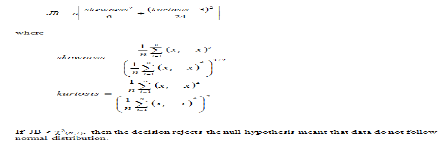
Where JB is the Jarque-Bera test statistic, n is the number of observations (or degrees of freedom in general) and S and K measures skewness and kurtosis of data respectively. To observe whether there is a normal distribution of data or not, the Jarque-Bera is applied which checks the chi-squared dispersion with two degrees of freedom. A JB value closer to zero shows that data is distributed normally.
Table 1 describes the descriptive statistics of NSE portfolio values, market price and conversion rate. The table reflects the main trend with the measurement of the mean, median and mode values. It measures the dispersion based on the value of variance and standard deviation. It also measures the normality of variables from kurtosis which estimates the perceptiveness of the spread of the time series. Skewness estimates the degree of freedom of the time series value. The values of kurtosis and skewness, indicate normal distribution as the kurtosis value of Indian market price is about 1 and the skewness value is about 0.56. If the kurtosis value of the conversion rate of both country, USD and Indian Rupees is lower than 1, it signifies a flatted curve. From the normal distribution, the JB (Jarque–Bera) statistic indicates the variance of the skewness and kurtosis of the time series value. An augmented Dickey-Fuller test (ADF) tests is a type of null hypothesis that a unit root is existent in a time series sample data analysis. The alternative hypothesis is diverse conditional on which account of the test is employed, but is frequently stationarity. It is an augmented description of the Dickey-Fuller test for a higher and more difficult set of time series models. To see the stationarity of the variables an augmented Dickey-Fuller (ADF) test has been used and it is a negative relationship. A stronger rejection of the hypothesis implies that there is a unit root existence at some level of confidence. The Augmented Dickey-Fuller adds lagged differences to these models:
| Table 1 Descriptive Statistics Values | ||
| Statistical tools | NSE Portfolio price (stock market price) | Conversion rate (USD and Indian Rupees) |
| Mean | 1863.5896 | 3.568952 |
| Median | 1756.5912 | 2.536891 |
| Maximum | 2135.5790 | 4.347268 |
| Minimum | 1420.7689 | 1.482451 |
| Std. dev. | 235.6931 | 0.536890 |
| Skewness | 0.563245 | 0.243719 |
| Kurtosis | 1.538627 | 1.528637 |
| Jarque–Bera | 5.356145 | 7.258963 |
| Probability | 0.000561 | 0.000147 |
| Sum | 21252.565 | 241.8524 |
| Sum sq. dev. | 2457575 | 4.258369 |
| Observations | 93 | 93 |
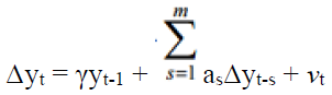
No constant, no trend:
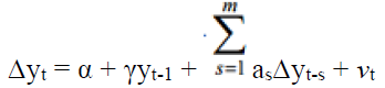
Constant, no trend:
Constant and trend:
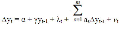
The Dickey-Fuller test establishes a simple autoregressive model by
Where yt is the variables below the research, t indicates time, α indicates the coefficient of variables and μtindicates the sampling error.
| Table 2 The Unit Root Test At Level | |||
| ADF unit root test at level | |||
| Variables | t-statistic | p-value* | Outcome |
| NSE Portfolio price | -1.586975 | 0.01415 | unsteady |
| Conversion rate (USD and Indian Rupees) | -0.869175 | 0.25836 | unsteady |
The above Table 2 shows the stationarity test results. The Indian financial market is non-stationary at a level with block and slacked indicated value “0”. The N0 hypothesis determines the Conversion rate (USD/INR) has a unit root, which indicates that it is not stationary at 5 per cent significance level.
| Table 3 The unit root test at the first difference level | |||
| ADF unit root test at first difference level | |||
| Variables | t-statistic | p-value* | Outcome |
| NSE Portfolio price | -4.258147 | 0.00014 | Steady |
| Conversion rate (USD and Indian Rupees) | -6.963147 | 0.00142 | Steady |
The above Table 3 shows that the significance of the unit root test. By taking the 1st difference all the variables got stationary at 1st difference. Further, the study has applied the Vector Auto Regress (VAR) method, variance decomposition and Granger Causality tests. VAR has been utilized to see the long-term combination of financial and economic factors.
Vector Autoregressive Model
Vector autoregressive model discusses the progression of a set of k variables (named endogenous variables) over the period from 2000 to 2019 (t = 1... T) The variables are together in a k-vector ((k × 1)-matrix) yt, which has as i th element, Yi,t, the number of observation at time t of the i th .. if the i th variable NSE Portfolio price, then yi,t is the value of Conversion rate (USD and Indian Rupees) at time t. A p-th order VAR, denoted VAR (p), is where there is the number of observations yt−i (i periods back) is called the i-th lag of y, c is a k-vector of constants (intercepts), Ai is a time-invariant (k × k)-matrix and et is a k-vector of error terms satisfying.
1. All error duration values have a mean zero;
2. The contemporary covariance matrix of error terms is Ω(a k × k positive-semi definite matrix);
3. For any non-zero k — there is no correlation across time; in particular, no serial correlation in individual error terms.
A p-order VAR is also known as a VAR with p lags. The procedure of selecting the maximum lag p in the VAR model necessitates special consideration because the implication is dependent on the correctness of the selected lag order. Vector autoregressive estimates NSE Portfolio price or stock market price and conversion rate (USD and Indian Rupees) in Table 4.
| Table 4 Vector Autoregressive Model | ||
| Variables | NSE Portfolio price | Exchange rate |
| Conversion rate (USD and INR) -1 | 0.173569 | -143.8695 |
| (0.852437) | (147.5815) | |
| [1.35146] | [-0.41218] | |
| Conversion rate (USD and INR) -2 | -0.008618 | 321.83190 |
| (0.531580) | (62.86137) | |
| [0.083127] | [0.206810] | |
| NSE Portfolio price -1 | 1.6815E-02 | 0.6025734 |
| (4.2852E-4) | 0.6347052 | |
| [0.3479510] | [2.025837] | |
| NSE Portfolio price -2 | -2.5361E-3 | -0.628152 |
| (3.02568E-2) | (0.538190) | |
| [0.230756] | [-0.581960] | |
| C | 2.3568E-1 | -2.560170 |
| (1.258963) | (8.369741) | |
| [-0.025803] | [-0.014706] | |
The VAR model was applied to see the relationship between stock market price and conversion rates. Granger causality, compulsion response purposes and difference disintegration expose approximately, how these variables move. The structural equation has also been used in this study. The two models developed with two variables NSE Portfolio price or stock market price and conversion rate (USD and Indian Rupees) D & INR (Conversion rate US_India) = C (1) * D & INR (Conversion rate US_India (-1)) + C (2) * D & INR (Conversion rate US_India (-2)) + C (3) * D & INR (NSE Portfolio price (-1)) +C (4) * D & INR (NSE Portfolio price (-2)) +C ...(1).
D & INR (NSE Portfolio price = C (6) * D & INR (Conversion rate US_India (-1)) + C (7) * D & INR (Conversion rate US_India (-2)) + C (8) * D & INR (NSE Portfolio price (-1)) +C (9) * D & INR (NSE Portfolio price (-2)) +C (10) .....(2).
The study has developed the Vector autoregressive estimates model with two dependant variables NSE Portfolio price and Conversion rate (USD and Indian Rupees). According to equation 1 and 2, there are 10 coefficients to determine the variables significance level at 1%, 5% and 10% level. The study can explore the results or outcome in the first equation that coefficient values end with C (5) and in the second equation, it begins with C (6) which indicates that this is a functional equation model which is associated with each other variables. To see whether the conversion rate (USD and Indian Rupees) lag 1 and lag 2 are significant to describe NSE Portfolio price, we have used the functional equation 1 and 2, it has explained in Table 5. The p-values of log 1 and log 2 are not significant to describe the NSE portfolio price. So, the study has used all variables without seeing the significant levels. Here, the conversion rate has lag 1 and it is significant because its p-value is less than 1% level and 5% level. Further, the response function has tested through Vector Autoregressive estimates. The instinct response always lies within the 95% coefficient interval.
VAR Estimation Method: Least-Squares System Equation
The least-squares method is used to estimate the determining systems. The greatest fit in the least-squares method is to minimise the sum of squared values. When the independent variable has spurious results, it is required to test the least-squares estimation.
The least-square line is named a Regression line.
y^= a + b x
Here, the stock price and conversion rate were used to see the dynamic relationship between these variables. To determine the outcome of the equation, the following steps are taken:
1. Stage 1: For each variable conversion rate and stock price (x, y) point to calculate x2 and XY.
2. Stage 2: Sum (x= conversion rate, y = stock price, and outcome of both variables x2 and xy, which values outcome has given the study Σx, Σy, Σx2and Σxy (Σ means "summation up")
3. Stage 3: Compute Grade m to m values = N Σ (XY) − Σx Σy N Σ(x2) − (Σx)2
4. Stage 4: Compute Divert b to b values = Σy − m Σx N.
5. Stage 5: Accumulate the equivalence of a least-square line intersecting with regression point.
| Table 5 VAR Estimation Method: Least Squares System Equation | ||||
| Variables | Coefficient | Std. error | t-Statistic | p-value |
| C (1) | 0.235 | 4.753 | -2.361 | 0.002 |
| C (2) | 0.147 | 4.318 | 0.428 | 0.042 |
| C (3) | 0.852 | 2.431 | -0.618 | 0.003 |
| C (4) | 0.351 | -0.617 | 0.403 | 0.360 |
| C (5) | 0.27E-01 | 0.718 | 0.108 | 0.021 |
| C (6) | -0.951 | -12.517 | -0.602 | 0.000 |
| C (7) | -0.753 | -3.819 | -0.861 | 0.541 |
| C (8) | -0.318 | -0.058 | 0.517 | 0.360 |
| C (9) | 0.24E-07 | 0.067 | -2.401 | 0.207 |
| C (10) | -0.849 | 0.001 | 0.951 | 0.096 |
| C (11) | -0.372 | -0.753 | 0.150 | 0.470 |
| C (12) | -0.68E-04 | 14.614 | -0.637 | 0.002 |
| C (13) | -0.95E-03 | 27.747 | 0.053 | 0.007 |
| C (14) | -23.851 | 10.327 | -1.036 | 0.230 |
| C (15) | -32.230 | 0.675 | -1.052 | 0.470 |
| C (16) | 1.568 | -8.348 | 0.860 | 0.001 |
| C (17) | -0.068 | 0.62E-05 | 0.753 | 0.008 |
| C (18) | 0.086 | -0.52E-01 | 0.510 | 0.537 |
| C (19) | -2.827 | -0.24E-07 | 2.023 | 0.672 |
Table 5 shows the shocks in the stock markets. It happened due to fluctuations in Indian Stock Market price, initially its diminutions the conversion rate in period 5 and 6 later it upsurges during period 7 and 8. The response of conversion rate assessment to the Indian stock market price level was perceived after 2010. When compared with the USD conversion rate, the INR conversion rate constantly deteriorated, the surprise or innovation of conversion rate level to the stock price originally has a perceptible effect on the Indian stock market price. It upsurges from 11 to 12 period and then slowly decreases being in the negative zone. In the short-term shockwaves, the exchange rate hurt the stock market price. Under the VAR model, the standard error and standard deviation have accepted levels. Inflation or financial crisis on stock market price harms the exchange rate as it inclines to escalation slowly and moves towards negative to from positive and becomes steady at zero. There is an interrelation between the two variables in the short term but in long term, there is no interrelation between the two variables.
| Table 6 Results of Variance Decomposition of Inr and Usd (Conversion Rate and Stock Market Price) | |||
| Years | INR and USD (Conversion rate) | Indian Stock market Price | SE |
| 2000 | 44.23 | 0.002 | 0.235 |
| 2001 | 47.45 | 0.230 | 0.425 |
| 2002 | 49.42 | 0.451 | 0.478 |
| 2003 | 50.67 | 1.235 | 0.985 |
| 2004 | 52.75 | 1.568 | 0.346 |
| 2005 | 53.68 | 1.746 | 0.304 |
| 2006 | 54.19 | 0.560 | 0.506 |
| 2007 | 56.75 | 1.860 | 0.806 |
| 2008 | 57.32 | 1.751 | 0.437 |
| 2009 | 57.91 | 1.307 | 0.521 |
| 2010 | 58.36 | 1.602 | 0.351 |
| 2011 | 59.37 | 1.948 | 1.603 |
| 2012 | 59.81 | 1.423 | 1.856 |
| 2013 | 60.39 | 1.602 | 0.527 |
| 2014 | 61.85 | 1.963 | 0.601 |
| 2015 | 64.16 | 1.852 | 0.750 |
| 2016 | 66.75 | 0.741 | 0.614 |
| 2017 | 67.85 | 1.342 | 0.527 |
| 2018 | 68.63 | 1.153 | 1.568 |
| 2019 | 70.08 | 0.749 | 2.509 |
The above Table 6 explains the variance decomposition analysis. It was done through the VAR approach. To run the VAR model the variables should be stationary at the first difference level. The lag selection criteria were done through AIC standards with 3 lags and finally, the VAR model was applied. The variance decomposition analysis was carried out with two endogenous variables; conversion rate and stock market price. Variance decomposition analysis provided a significant outcome. The study can forecast frequently incidental from past trends. There are two important activities, which are short term and long-term. In the short term, the individual conversion rate fluctuations record 49.42%, compulsion or invention or surprise towards the financial conversion rate records. In the long-term fluctuations of stock market price impacted at 0.451%, the variation in the conversion rate of India with a comparison of USD. The circumstance represents a short-term balance between the two variables. Between these two variables, there is an influence but the amount of effect is a bit high.
| Table 7 Results of Var Granger Causality Test/Block Homogeneity Wald Tests (Sample Data: from 2000 to 2019) | |||
| Depended Variable: conversion rate (INR and USD) | |||
| Excluded | Chi-sq. value | Df (Degree of freedom) | p-value |
| Indian Stock market price | 1.25368 | 3 | 0.0675 |
| All | 3.56781 | 3 | 0.3421 |
| Depended Variable: Indian Stock market Price | |||
| Excluded | Chi-sq. value | Df (Degree of freedom) | p-value |
| conversion rate (INR and USD) | 7.95471 | 3 | 0.2274 |
| All | 5.27140 | 3 | 0.0317 |
The above Table 7 explains the outcome of the VAR and Granger causality test. Here, the conversion rate and the Indian stock market prices are the dependent and the independent variable respectively. Here, we frame the N0 hypothesis and the results show that in the short-term conversion rate does not depend on the Indian stock market price. It declares that it hurts macroeconomic factors. The p-value indicates that it is more than the 5% significant level and the N0 hypothesis cannot be approved which assumes that the conversion rate doesn’t influence stock market price because it has negative results. Further, it has considered testing the alternative hypothesis. Here, we have exchanged the variables in the opposite direction, i.e stock market price is a dependent variable whereas the conversion rate is chosen as an independent variable. The alternative hypothesis shows that the Indian conversion rate is not impacted positively by the stock market price. Further, it has observed that the p-value is less than the 5% significant level and it has proved the alternative hypothesis and disapproved the null hypothesis. Therefore, there is a condition that the conversion rate has a positive impact on stock market price and there is no causal relationship among these variables.
Conclusion
The study has analysed the relationship between the Indian stock market price and conversion rate. We have applied the unit root tests, VAR approach, Granger causality test and variance decomposition methods in the short term and long term. The study shows that in the long-term Indian stock market price and the conversion rate has a positive impact, whereas in the short term there is a negative impact on the macroeconomic factors. The present position of the Indian financial market shows a negative trend and the overall financial position has drastically reduced. Inflation is gradually increasing. To understand the fundamentals which are distressing business segments, the financial market has resolved out to be uncomplicated. This approach is not only being applied in India but at the international level as well.
The VAR estimation shows that in the short term, there is a relationship between the conversion rate and the Indian stock market. Further, it leads to the compulsion response function and variance decomposition under the VAR model. The results indicate a negative relationship between these two variables which is statistically significant in the short term but in the case of the long term, they are highly insignificant. In the short term, the degree of association between conversion rate and Indian stock market price has a low impact. There is no long-term cointegration between conversion rate and market price. The results are supported by the Indian Stock market price, which is the maximum returns of share values. Finally, there is no long-term integration between conversion rate and stock market price. The VAR and Granger causality observes that there is no causal relationship between these two variables. The study also provides supplementary captivation. The stock market and conversion rates are prejudiced by macroeconomic indicators in the developed nation’s stock exchange. Further, the study can be used equally to focus on the close exploration of generating results in the financial market and reformed markets.
References
- Choi, Y.K., & Kim, D. (2000). Determinants of American Depositary Receipts and their Underlying Stock Returns Implications for International Diversification. International Review of Financial Analysis, 9, 351- 368.
- Damele, M., Kannarkar, Y., & Kawadia, G. (2004). A Study of Market Integration based on Indian Stock Market, Bullion Market and Foreign Exchange Market. Finance India, XVIII(2), 859-869. doi:10.1080/23322039.2018.1432450.
- Granger, C.W., Huangb, B.N., & Yang, C.W. (2000). A bivariate causality between stock prices and exchange rates: Evidence from recent Asianflu. The Quarterly Review of Economics and Finance, 40(3), 337–354. doi:10.1016/S1062-9769(00)00042-9
- Habib, M., & Stracca, L. (2012). Getting beyond carrying trade: What makes a haven currency? Journal of International Economics, 87, 50–64.
- Jayasuriya, S.A. (2011). Stock market correlations between China and its emerging market neighbors. Emerging Markets Review, 12(4), 418-431. doi: 10.1016/j.ememar.2011.06.005.
- Jithendranathan, T., Nirmalanadan, T.R., & Tandon, K. (2000). Barriers to lnternational Investing and Market Segmentation: Evidence from Indian GDR Market. Pacific-Basin Finance Journal, 8, 399-417.
- Magda, K., & Ida, M. (2005). The Effects of Exchange Rate fluctuation onOutput and Prices: Evidence From Developing Countries, The Journal of Developing Areas, 38(2), 189-219.
- Megaravalli, A.V., & Sampagnaro, G. (2018). Macroeconomic indicators and their impact on stock markets in ASIAN 3: A pooled mean group approach. Cogent Economics & Finance, 6(1), 1432450.
- Moore, T., & Wang, P. (2014). Dynamic linkage between real exchange rates and stock prices: Evidence from developed and emerging Asian markets. International Review of Economics & Finance, 29, 1-11. doi:10.1016/j.iref.2013.02.004.
- Nenavath, S. (2019). An econometric time-series analysis of the dynamic relationship among trade, financial development and economic growth in India. Asian Economic and Financial Review, 9, 155-165.
- Nenavath, S. (2018). An Empirical Test of Capital Asset-pricing Model and Three-factor Model of Fama in Indian Stock Exchange. Management and Labour Studies, 43(4) 1-14, SAGE Publications sagepub.in/home.nav DOI: 10.1177/0258042X18797770, http://journals.sagepub.com/home/mls.
- Ono, S. (2017). Financial development and economic growth nexus in Russia. Russian Journal of Economics, 3(3), 321-332. doi:10.1016/j.ruje.2017.09.006.
- Priestley, R., & Odegaard, B.A. (2004). Exchange Rate Regimes and the Price of Exchange Rate Risk, Economic Letters, 82, 181-188.
- Purbaya, & Yudhi, S. (2000). The effect of exchange rate on foreign direct investment Dissertations, Purdue University, Journal of Finance, 71(2).
- Rashmi, C., Dheeraj, M., & Priti, B. (2020). Conditional relation between return and co-moments – an empirical study for emerging Indian stock market. Investment Management and Financial Innovations, 17(2), 308-319. doi:10.21511/imfi.17(2).2020.24.
- Shamsuddin, A.F.M., & Kim, J.H. (2003). Integration and Interdependence of Stock and Foreign Exchange Markets: An Australian Perspective. Journal of International Financial Markets, Institutions and Money, 13, 237-254.
- Shankar, R.L., Ganesh, S., & Kiran, K. (2019). Mispricing in Single Stock Futures: Empirical Examination of Indian Markets, Emerging Markets Finance and Trade, 55(7), 1619-1633, DOI: 10.1080/1540496X.2018.1477681
- Tomoe, M., & Eric, J.P. (2006). the Sources of Real Exchange Rate Fluctuations in India, Indian Economic Review, New Series, 41(1), 9-23.