Keywords

PCA, Eigen Values, Eigen Vector, Bond Yield, Hedging, DV01.

Introduction

The modern business and policymaking environments are driven by the players' ability to utilize the vast amounts of information available to make competent decisions. In the financial market domain mainly, an increasingly large volume of data is generated every day. The advent of powerful machine learning and big data technologies makes it easy for financial analysts to promptly get high-quality financial market information and forecasts. However, in some cases, data that contains too many dimensions or features may lower the accuracy of a model because it presents the machine learning algorithms with overwhelming datasets to be generalized (Guo et al., 2015). This may lead to inaccurate forecasts as the algorithms attempt to fit all the dataset's features into a model. To address this problem, ways of reducing data dimensionality have been developed to curb the challenges of overfitting and the complexity of large datasets (Mosetti, 2016). This can be achieved using feature selection or feature extraction (Sabău-Popa et al., 2020). Feature selection involves choosing a subset of the original features by expelling redundant features using variance thresholds. In contrast, feature selection involves generating new features from the original data using principal component analysis (PCA). This paper examines PCA and applies it to determine an effective hedging strategy of a Treasury bond portfolio using a given dataset.

Application of Principal Component Analysis (PCA)

Principal component analysis (PCA) is a mathematical technique of dimensionality reduction by transforming correlated input data into an uncorrelated output dataset whose explained information or variance is maximized. Therefore, PCA reduces the dimensionality of an input dataset while also ensuring that it preserves maximum information (NiketBorade & Deshmukh, 2014). The justification of using PCA is that it is possible to take advantage of the correlations between the variables in a high dimension-population system to create a smaller dimension-population system that can produce a yield curve model with a comparable level of predictive accuracy (Papi & Caracciolo, 2018). This conceptualization arises from evidence-based knowledge that the movements of adjacent points on a financial market yield curve are not independent. PCA exploits this interdependent movement of points to identify reduced dimensionality models that, although they may reduce accuracy, make the data more straightforward and faster for forecasting algorithms to process (Kwong & Mak, 2017).

A principal component (PC) is a vector of a variable, such as the forward rate of the yield of a treasury bond. When presented on a yield curve, the first PC is considered to carry the most weight in capturing variance with the weight-reducing for each subsequent PC ( Tran & Osipenko, 2016). PCs are obtained through eigenvalue decomposition of the covariance or correlation matrix of a stock market portfolio. Therefore, PCs are the vectors of the possible deviations of forward rates from the mean rate (Tharwat, 2016). Yield curves usually evolve stochastically, featuring multiple possible stochastic differential equations, which are substantially complex to model and predict when the entire universe of possible curves from the total population is considered (Kelly et al., 2017). The goal of PCA is to minimize the dimensions of the dataset to obtain a set of PCs that explain the highest percentage of the yield curve variability (Abdi & Williams, 2010). For example, the figure below Figure 1 represents the yield curves of the USD economy as of 31st December 2012. The figure on the right represents 10,000 possible yield curves based on a two-factor Black-Karasinski stochastic model, while the first figure shows a reduced yield curve of the population (Redfern & McLean, 2014). Both scenarios represent 50 forward rate yield curves. Forecast modeling using the total population of yield curves would be complex and result in overfitting.

To obtain the reduced yield curve, the three most significant PC yield curves from the population were obtained through eigenvalue decomposition and identification of Eigenvectors. An Eigenvector occurs at the point of orthogonal or perpendicular intercept between a base PC linear curve, starting from the origin of the curve axis, and another PC curve (Sang, Wang & Cao, 2017). The eigenvalue, then, is the variance between the point of intercept and the mean yield curve Figure 2.

The normalized PC yield curves were obtained and then scaled according to their significance from the previous example, as shown below (Figure 3). In the scaled version shown in the second diagram, the blue PC curve explains the highest variability of 91%. The second PC curve represents a tilt in the yield curve, presenting 8.3% of the variance. The third PC curve can be defined as a higher-order buckling capturing only 0.31% variability (Redfern & McLean, 2014). Therefore, to achieve the objective of dimensionality reduction, the first and second PC curves are sufficient for modeling the reduced yield curve since they capture approximately 99.3% variability in the yield curve.

To develop a full statistical reduced model of the universe, the yield curve based on the forward rate mean value is plotted and the possible subspace determined by plotting the maximum eigenvalues of the essential PCs above and below the mean yield curve in the direction of the Eigenvectors (Jiang, 2016) as shown in the figure below. The solid curve represents the mean yield curve, while the broken curves are the maximum variances of the curve as dictated by the most significant PCs.

The equation for the forecasted forward rates Fj according to the statistical model between j and j + 1 years are represented by the equation:

F = µ + α1v1,j

Where µ is the mean forward yield rate at time t = 1, α1 is the scaling value of the most significant PC curve, and v_{i, j} is the jth value of the most considerable PC curve.

The equation can be presented in vector terms as:

F = µ + α1v1

Where F represents all forward yield rates, µ represents all mean values, and v1 represents all Eigenvectors making up an essential PC curve. Given the significance of the first PC curve that captures 91% of variability, its shape above and below the mean yield curve explains the shape of the yield curve universe (Redfern & McLean, 2014). Using the statistical model, including more PC curves into the model, one can generate the desired universe of as many yield curves as possible.

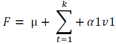
The full statistical model can be presented as:

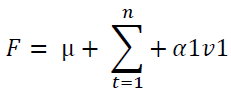
While the reduced statistical model can be presented as:

Application of PCA in Finance

PCA analysis is a vital technique for helping investors and analysts decompose the movements in portfolio yield curves, analyze, and describe them to understand the risks involved in various investments and how to anticipate or mitigate them. The primary basis of PCA is that movements in yield curves are caused by interdependent movements in adjacent points within a population of yield rates following structural stochastic models (Liu & Wang, 2011). However, given the sheer volume of data generated in financial markets, using a universe of data to develop predictive models is too complex and may lead to model overfitting. PCA helps analysts and investors to simplify these models to obtain simpler predictive models that are also easier for supervised machine learning algorithms to process. PCA is a popular method that leads to high levels of accuracy due to its focus on feature extraction instead of feature selection. Feature extraction exploits entire datasets to achieve a dimensionality reduction, while feature selection incorporates filtering tactics to obtain subsets of data (Liu & Wang, 2011). Consequently, by relying on complete datasets and attempting to retain as much information as possible, the feature extraction approach of PCA is superior to feature selection techniques.

The traditional approach to hedging assumed that parallel shifts in portfolio yield curves are necessary for developing risk management strategies. However, recent studies have revealed that financial market yield curves follow complex stochastic models, which imply that they are likely to frequently display non-parallel shifts (Lin et al., 2015). Although this approach may have been valid in the early years of modeling financial market behavior, the modern environment is highly complex. It cannot support the linear models that were prevalently applied in traditional approaches. Such models tend to oversimplify financial markets and do not consider the numerous factors in the modern setting that affect the performance of financial instruments. For example, the famous Standard & Poor's (S&P) 500 Index changes its composition regularly due to diverse factors ranging from company-specific performance to macroeconomic factors (Liu & Wang, 2011). The governing committee of the S&P 500 Index appreciates that financial markets follow non-linear patterns that simplistic linear models cannot represent, thus, discrediting the assumption of parallel shifts in yield curves as hypothesized by traditional risk management models.

Alternatively, the PCA method seeks to identify a few factors that affect non-parallel shifts in yield curves as possible and use those factors to develop predictive models. The model has an advantage over more modern approaches such as the three-factor model. It views movements in adjacent points on a yield curve as correlated and seeks to transform them into an uncorrelated relationship (Liu & Wang, 2011). The establishment of independence in the output eliminates the risk of factor relationship, which is a challenge in other methods such as the three-factor technique. As a result, the PCA approach provides a highly comprehensive means for analysts and investors to craft hedging strategies and reduce risks.

Interest Rate Risk Management in a Bond Portfolio

The dollar value of a 01 (DV01), also called the present value of 01 (PV01), refers to the change in the value of financial security, such as a bond, for a basis point change of 0.0001 in interest rates. DV01 is measured in the nominal change in dollars and is not expressed as a ratio or percentage. As a result, DV01 provides investors and analysts with the evolution of a bond's price in dollars based on the 0.0001-point change in its yield to maturity relative to interest rates (Chertok, 2012). Since the primary goal of hedging is to lock in a bond's present position regardless of any changes in its maturity yield, the par amount for selling or buying a bond's hedge position for every $1 par value is determined by the hedge ratio based on the original position (Cesari & Mosco, 2017).

The effective duration of a bond measures the sensitivity of a bond's prices in relation to interest rate fluctuations while considering variables such as final maturity periods in years, yields, calls, coupons, and present values. The risks involved in determining the maturity yield of bonds increase with time due to the negative correlation between interest rates and bond prices (Cesari & Mosco, 2017). This implies that a fall in interest rates increases the prices of bonds while a rise in interest rates adversely affects bond prices the risks involved in this relationship increase over time. The interpretation of the increase in a bond's risk as its duration increases is that an investor is compelled to wait for a longer time to recoup their principal investment and yield for a long maturity bond subject to changes in interest rates as compared to a short maturity bond whose price will not fall as much in case of a rise in interest rates (Cesari & Mosco, 2017).

The duration of a bond refers to the inverse linear relationship between interest rates and bond prices. The linear relationship is a suitable method of measuring the sensitivity of bond prices to changes in interest rates but only for small yield fluctuations. When bond yield fluctuations are large, the relationship between bond prices and interest rates becomes non-linear, making duration an unreliable measure of sensitivity (Cesari & Mosco, 2017). This non-linear relationship for large yield fluctuations is called convexity. A combination of both measures provides a more accurate estimation of the percentage changes in bond prices due to a certain percentage change in bond yield compared to using duration alone.

Process and Methodology

Data

We took a constant maturity yield of Treasury bonds and plotted the historical five-year yield. Data itself looks correlated, at least for the adjacent maturity, as shown below Figure 4.

The process and methodology of performing PCA to develop hedging strategies can be shown using a time series data from NASDAQ containing the yields of 9 Treasury bonds of 1 month, three months, six months, one year, two years, three years, five years, seven years, and 20 years maturities. For this report, it was assumed that the Treasury bonds in the portfolio are held equally and that each has an 11.11% representation in the portfolio. The PCA computation is done using StatistiXL software. Before using the StatistiXL software, the data were examined to ensure that it was complete and continuous. A summary statistic has been extracted.

The next step is the computation of the correlation matrix. A correlation matrix was chosen because the bond yields have different variances. The correlation matrix is necessary for measuring whether there are relationships between the yields of the various bonds. This helps to identify any redundant information that may arise from high levels of correlation between the variables.

The further step is the extraction of eigenvalues and eigenvectors from the correlation matrix from which the PCs will be computed. The main goal of PCA is to generate a new set of values, called PCs, which ensure the least correlation between the variables. PCs are a product of linear combinations of the initial variables to create the uncorrelated variables. There are as many PCs as the number of variables. Thus, the data used in this paper will generate 9 PCs. PCs are then arranged such that the first PC explains the most significant variance in the dataset, and the value of explained variance reduces with each subsequent PC. Calculating the cumulative percentage of variance starting with the first PC makes it possible to identify the set of PCs that explain the most variance and the corresponding bonds that need to be hedged. This paper aims to capture the first set of PCs that explain at least 97% of the bond yield variance.

To interpret the results of the PCA, a computation of the correlations between the principal components and the initial variables is required. The correlations are calculated using a correlation technique called component loading. The correlation between the two is evaluated to determine the degree of variance that a PC explains about a variable. The variables whose variance is explained the largest by the PCs are the highest correlations with the PCs. Since the correlation between independent PCs and the variables varies, choosing the most significant variables is a subjective decision. For this paper, the essential variables will be those that PC1 is most correlated to.

Results and Interpretation

The descriptive statistics of the dataset are as follows Table 1:

Table 1 Descriptive Statistics of the Dataset
Variable	Mean	Std Dev.	Std Err	N
1M	1.069	0.842	0.024	1226
3M	1.127	0.845	0.024	1226
6M	1.235	0.828	0.024	1226
1Y	1.341	0.800	0.023	1226
2Y	1.502	0.726	0.021	1226
3Y	1.635	0.664	0.019	1226
5Y	1.875	0.579	0.017	1226
7Y	2.086	0.527	0.015	1226
20Y	2.530	0.433	0.012	1226

The correlation matrix of the portfolio is as follows Table 2:

Table 2 Correlation Matrix
	1M	3M	6M	1Y	2Y	3Y	5Y	7Y	20Y
1M	1.000	0.996	0.987	0.963	0.906	0.842	0.694	0.566	0.329
3M	0.996	1.000	0.996	0.979	0.930	0.872	0.733	0.609	0.372
6M	0.987	0.996	1.000	0.992	0.955	0.905	0.777	0.659	0.424
1Y	0.963	0.979	0.992	1.000	0.983	0.946	0.838	0.732	0.502
2Y	0.906	0.930	0.955	0.983	1.000	0.988	0.918	0.834	0.627
3Y	0.842	0.872	0.905	0.946	0.988	1.000	0.967	0.906	0.729
5Y	0.694	0.733	0.777	0.838	0.918	0.967	1.000	0.984	0.871
7Y	0.566	0.609	0.659	0.732	0.834	0.906	0.984	1.000	0.942
20Y	0.329	0.372	0.424	0.502	0.627	0.729	0.871	0.942	1.000

All the variables show positive correlations. The results of the extraction of eigenvalues and the corresponding PCs are as follows Table 3:

Table 3 Explained Variance (Eigenvalues)
Value	PC 1	PC 2	PC 3	PC 4	PC 5	PC 6	PC 7	PC 8	PC 9
Eigenvalu	7.567	1.356	0.065	0.008	0.003	0.001	0.001	0.000	0.000
% of Var.	84.075	15.062	0.717	0.084	0.035	0.013	0.008	0.003	0.003
Cum. %	84.075	99.137	99.854	99.938	99.973	99.986	99.994	99.997	100.000

From these results, we can determine the PCs that explain the most significant variance of bond yields. PC1 explains the most considerable variance of the bond yields of 84.075%, followed by PC2 at 15.062% Figure 5. Cumulatively, the first two PCs explain 99.137% of all variance of the Treasury bond yields, surpassing the rule of 97% used as the benchmark for this paper.

The correlations between the first two PCs and the variables are as follows Table 4:

Table 4 Component Loadings (Correlations Between Initial Variables and Principal Components)
Variable	PC 1	PC 2
1M	0.897	-0.426
3M	0.921	-0.382
6M	0.945	-0.323
1Y	0.972	-0.227
2Y	0.993	-0.059
3Y	0.991	0.089
5Y	0.939	0.335
7Y	0.868	0.495
20Y	0.686	0.710

From these results, the first PC has a high positive correlation with all the variables as the PC that explains most of the variance in bond yields implies that the likelihood that the yields of all the Treasury bonds vary together. The three highest correlations are between PC1 and the two years maturity bond (0.993), the 3-year maturity bond (0.991), and the 1-year maturity bond (0.971). On the other hand, PC2 is negatively correlated to 5 of the initial variables. However, since PC2 explains only 15.062% of all variance in bond yields, the implication of PC1 is that the yields of all the Treasury bonds change together may still hold. PC2 is positively correlated to only 4 of the variables, namely the 3-year (0.089), 5-year (0.335), seven-year (0.495), and 20 years (0.710) maturity bonds. The most correlated bonds are the 20 years (0.710), seven-year (0.495), and five years (0.335).

The analysis of the component loadings can be used to determine the set of 2 or 3 Treasury bonds that are most affected by the variance explained by PC1 and PC2. While the highest correlations between the first two PCs and the initial variables point to different bonds, estimating the bonds that bear the largest explained variance is possible. PC1 and PC2 concurrently have positive correlations with four variables: the 3-year, 5-year, seven-year, and 20-year maturity bonds. The three highest correlations of the four for PC1 are the 3-year (0.991), 5-year (0.939), and 7-year (0.868) maturity bonds, while for PC2 are the five-year (0.335), seven-year (0.495), and 20 years (0.710). Therefore, the two bond yields for which PC1 and PC2 explain the most variance are the five-year and 7-year bonds.

Therefore, the most effective hedging strategy for the Treasury bond portfolio is to hedge the five-year and 7-year maturity bonds.

Conclusion

The advent of powerful machine learning and big data technologies makes it easy for financial analysts to promptly get high-quality financial market information and forecasts. However, in some cases, data that contains too many dimensions or features may lower the accuracy of a model because it presents the machine learning algorithms with overwhelming datasets to be generalized. To address this problem, ways of reducing data dimensionality, such as principal component analysis (PCA), have been developed to curb the challenges of overfitting and the complexity of large datasets.

PCA is a mathematical technique of dimensionality reduction by transforming correlated input data into an uncorrelated output dataset whose explained information or variance is maximized. Therefore, PCA reduces the dimensionality of an input dataset while also ensuring that it preserves maximum information. A principal component (PC) is a vector of a variable, such as the forward rate of the yield of a treasury bond. When presented on a yield curve, the first PC is considered to carry the most weight in capturing variance with the weight-reducing for each subsequent PC. Yield curves usually evolve stochastically, featuring multiple possible stochastic differential equations, which are substantially complex to model and predict when the entire universe of possible curves from the total population is considered. The goal of PCA is to minimize the dimensions of the dataset to obtain a set of PCs that explain the highest percentage of the yield curve variability.

The traditional approach to hedging assumed that parallel shifts in portfolio yield curves are necessary for developing risk management strategies. However, recent studies have revealed that financial market yield curves follow complex stochastic models, which imply that they are likely to display non-parallel shifts frequently. Such models tend to oversimplify financial markets and do not consider the numerous factors in the modern setting that affect the performance of financial instruments. The primary basis of PCA is that movements in yield curves are caused by interdependent movements in adjacent points within a population of yield rates following structural stochastic models. The model has an advantage over more modern approaches such as the three-factor model. It views movements in adjacent points on a yield curve as correlated and seeks to transform them into an uncorrelated relationship. The establishment of independence in the output eliminates the risk of factor relationship, which is a challenge in other methods such as the three-factor technique.

This paper conducted PCA on a dataset from NASDAQ of 9 Treasury bonds with different maturity periods to determine an effective hedging strategy. The computations performed on the data include descriptive statistics, correlation matrix, explained variance using eigenvalues, component loading, and a scree plot. The extraction of eigenvalues and eigenvectors from the data produced 9 PCs, of which the first two explain 99.137% of all variance in the bond yields. Analyzing the correlations between the first two PCs and the initial variables revealed that the best bonds to hedge in the portfolio are the five-year and 7-year maturity bonds. Further research is recommended to develop a statistical method of determining the best bonds to hedge based on the component loading tables.

References

Abdi, H., & Williams, L. (2010). Principal component analysis. Wiley Interdisciplinary Reviews: Computational Statistics, 2(4), 433-459.

Cesari, R., & Mosco, V. (2017). Duration, Convexity, and the Optimal Management 0f Bond Portfolios for Insurance Companies. SSRN Electronic Journal.

Chertok, D. (2012). Practical Yield, Price, Duration and Convexity Approximations. SSRN Electronic Journal.

Guo, Z., Wang, H., Yang, J., & Miller, D. (2015). A Stock Market Forecasting Model Combining Two-Directional Two-Dimensional Principal Component Analysis and Radial Basis Function Neural Network. PLOS ONE, 10(4), e0122385.

Jiang, H. (2016). Modularity Component Analysis versus Principal Component Analysis. American Journal of Applied Mathematics, 4(2), 99.

Kelly, B., Pruitt, S., & Su, Y. (2017). Instrumented Principal Component Analysis. SSRN Electronic Journal.

Kwong, R., & Mak, R. (2017). Examining Systematic Risk with Principal Component Analysis: An Empirical Analysis in Hong Kong Stock Market. Journal of Business and Policy Research, 12(2), 1-13.

Lin, Z., Wang, L., & Cao, J. (2015). Interpretable functional principal component analysis. Biometrics, 72(3), 846-854.

Liu, H., & Wang, J. (2011). Integrating Independent Component Analysis and Principal Component Analysis with Neural Network to Predict Chinese Stock Market. Mathematical Problems In Engineering, 2011, 1-15.

Mosetti, R. (2016). Principal Component Analysis of quantum correlation. The European Physical Journal Plus, 131(12).

NiketBorade, S., & R. Deshmukh, R. (2014). Comparative Study of Principal Component Analysis and Independent Component Analysis. International Journal Of Computer Applications, 92(15), 45-49.

Papi, M., & Caracciolo, G. (2018). Principal component analysis of personalized biomolecular corona data for early disease detection. Nano Today, 21, 14-17.

Redfern, D., & McLean, D. (2014). Principal Component Analysis for Yield Curve Modelling: Reproduction of out-of-sample yield curves. Retrieved from https://www.moodysanalytics.com/-/media/whitepaper/2014/2014-29-08-PCA-for-Yield-Curve-Modelling.pdf

Sabău-Popa, C., Simut, R., Droj, L., & Bențe, C. (2020). Analyzing Financial Health of the SMES Listed in the AERO Market of Bucharest Stock Exchange Using Principal Component Analysis. Sustainability, 12(9), 3726.

Sang, P., Wang, L., & Cao, J. (2017). Parametric functional principal component analysis. Biometrics, 73(3), 802-810.

Tharwat, A. (2016). Principal component analysis - a tutorial. International Journal Of Applied Pattern Recognition, 3(3), 197. Tran, N., & Osipenko, M. (2016). Principal Component Analysis in an Asymmetric Norm. SSRN Electronic Journal.