Keywords

Distance to Default, Probability of Default.

Introduction

Predictions about corporate default can only be made with a certain degree of probability, it is never certain. A firm's default probability can be very low, but it is never zero. In contrast, if default occurs, it will cause financial damage to the lender, so determining the possibility of default is an important and necessary issue. Researchers and organizations have been predicting the probability of failure for decades. The probability of default can be simulated in different ways and also by using different models. These models evaluate probabilities using market and fundamental data can be divided into two groups based on different assumptions, so the article distinguishes between structural models and reduction models (Katarína, 2011). Developed hybrid models to try to integrate assumptions from both previously mentioned models, structural and reductionist approaches.

Valuation models view the equity of the firm as a call option on the underlying asset. Because at the maturity of the debt, bondholders receive the debt and shareholders hold the remainder. Assumptions based on usage (Delianedis, 2003) observable value (VE) and volatility of equity E (volatility of equity), unacceptable value VA (unobservable) value) and the volatility of the firm's asset A (asset), Black and Scholes' option pricing theory, call capital on the firm's asset value – VA is considered as C, VE as C, D (debt) debt is exercised as a strike price, so D is treated as K (Kollár & Gond?árová, 2015). The origins of structural models have been traced back to the publications of (Fischer Black & Scholes, 1973) and (Merton, 1974). (Geske, 1979) then derived Merton's assumptions by looking at the many possible default options for coupons, sinking funds, debt, safety covenants, or other possible payment obligations. considered as the most suitable option. Another way is to demonstrate that it allows for reduced refinancing and limits on refinancing. Another aspect (Eom et al., 2002) also makes a different assumption about the same structural model (Lando, 2004). The article mentions that calculating the distance to default is part of the KMV model introduced by Kealhofer et al. (1974), which is also an extension of Merton's model and demonstrates the approach structure.

Literature Review

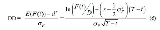
The KMV model was established as mentioned above by Keaholfer, McQuown and Vasicek in 1974 and is based on the assumption of Merton's bond price model. Then, in 2002, it was purchased by Moody's. They had some expectations of creating commercially acceptable credit methods. The main difficulty, as in other structural models, is how to assign dynamics to firm value, which is an unobservable process. The KMV model estimates the probability of default for each firm in the example at any given time. To estimate the probability of default, the model deducts the face value of the firm's debt from an estimate of the firm's market value and then separates this difference by an approximation of the variable firm action. The resulting z-score is known as the distance to default, and it then substitutes for a cumulative density function to calculate the probability that the firm's value will be less than the face value of the debt while critical path forecasting.

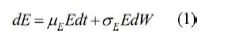
Where μE and σE are the expected return on equity and its volatility. The volatility of equity can be calculated by the following formula:

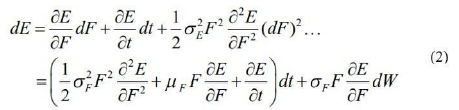
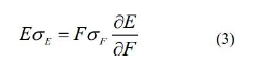
From equations (1) and (2), we have the following equality:

Combined with the option pricing formula in Merton's option theory model:

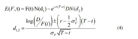
To calculate the market value of a firm, simply calculate the sum of the market values of the firm's debt and the value of its equity. Calculating the probability of default is simpler while both of these quantities are observable. Although an equity value is frequently available, reliable data on the market value of a firm's debt is not always available based on financial statements and information from credit firms. CIC national used This model is based on estimating the assets of the firms, that is, the present value and the change value from the market value of the equity of the firm and the instantaneous change in equity. ownership, along with knowing the excellence and maturity of debt. The maturity of the debt is chosen and the book value of the debt is set to be equal to the face value of the debt. Corporate default then occurs when the value of the firm's assets falls to the default point, which is the face value of the debt (Kollár, 2014). To quantify the probability of default using the KMV model, we introduced the new variable distance to default, which represents the gap between the expected value of the firm's assets and the default score, and then Divide this difference by estimating the volatility of the firm over a period of time. At that time, the distance to default is substituted for an accrual density function to calculate the probability that the value of the firm will be less than the face value of the debt at the maturity of the debt (Ammann and Manuel, 2001). Based on Merton's assumption, equity is viewed as a call option given the firm's asset value and time. Thus, it follows the following stochastic equations: The value of equity for public firms can be observed directly from the stock market, since it directly suggests that the value of the stock option option written on the underlying value of the firm's assets can be observed. Alternatively, the volatility of equity can be obtained by approximating the implied volatility from an observed option value or by using stock return data. Once we have the interest rate risk and the maturity of the debt, the unknown index is the asset value of the firm F (t) and the volatility of the firm σF. Thus, the two nonlinear equations (3) and (4) can then be solved by determining F (t) and σF in terms of equity value, volatility value and capital structure.

Methodology

The KMV model violates (Merton, 1974)'s assumption that a firm's assets are tradable so that it realizes this point. The KMV model uses Black-Scholes and Merton constructs as inspiration to calculate an intermediate period known as the distance to default and then calculates the probability of default. First, the distance to default should be calculated and can then be developed and estimate the probability of default of a particular firm as a result of the asset value of the firm and the volatility of its assets (Black, 1973). A default event occurs when the value of a firm's assets falls below the default point. In Merton's model, the face value of debt is observed as the default point, and the distance to default can be calculated by using the volatility of the firm's assets. The chance that a firm will default is less when the number of default intervals is higher (Kliestik et al., 2015).

d* = Short-term debt + ½ Long-term debt .....(5)

Inside:

DD: Distance to default r: the asset's risk-free rate

F(t): short-term asset value D: face value of debt

σF: volatility of firm value

The study focuses on steel companies listed on the Vietnamese stock market to calculate the distance to default according to KMV's model (Kealhofer et al., 1990).

Research data according to five periods from 2010 to 2019. This study uses a quantitative method through statistical probability theory. The probability distrifirmtion is considered suitable for the data tested through POLS model, FE test, RE test with the support of simulation software.

Result, Analysis and Discussion

Among the industrial production industries, the steel industry is strongly affected by the impact of the economic crisis because it is both strongly influenced by the domestic market and strongly influenced by the foreign market. Raw materials must be imported. Steel firms always face difficulties and challenges. The risk of default of steel firms also increases accordingly. Factors affecting the risk of default of a firm can be mentioned as follows:

Firm of distance to default (DD), return on total assets (ROA), return on equity (ROE), current assets, long-term assets, liabilities.

The POLS model results suggest that: DD ~ lag(DD, 1) + ROA + ROE + SOA + log(X5) + log(X27) + log(X59) with value Chisq là 3.4179 and P-value is 0.06449.

orrection of RE . model ## t test of coefficients:

## Estimate Std. Error t value Pr(>|t|)

## (Intercept) 9.845525 1.336900 7.3644 2.620e-11 ***

## lag(DD, 1) 0.037039 0.118303 0.3131 0.75476

## ROA 0.454907 0.457431 0.9945 0.32202

## ROE-0.140859 0.070118 -2.0089 0.04683 *

## SOA 0.154548 0.160737 0.9615 0.33827

## log(X5) -0.063757 0.268345 -0.2376 0.81261

## log(X27) 1.279505 0.167810 7.6247 6.834e-12 ***

## log(X59) -1.707861 0.293775 -5.8135 5.321e-08 ***

## Signif. codes: 0 '***' 0.001 '**' 0.01 '*' 0.05 '.' 0.1 ' ' 1

So from the above results, we have a model of factors affecting the distance to default of steel firms listed on the Vietnamese stock market. The results are as follows:
DD = 9.845525 + 0.037039*lag(DD,1) + 0.454907*ROA – 0.140859 *ROE +0.154548*SOA– 0.063757*log(X5) + 1.279505*log(X27) – 1.707861*log(X59)

Inside

lag(DD,1): lagged variable, previous period of DD to account for current variable ROA: Return on total assets = X165/X57

ROE: Return on equity = X165/X59

SOA: Equity/total assets or financial leverage = X79/X57 log(X5): Logarit short-term assets

log(X27): Logarit long-term assets log(X59): Logarit long-term loans and debt

Result, Analysis and Discussion

Firstly, the liabilities of the firm are inversely proportional to the distance to default. The reason is that if the creditors give the firm a lot of debt for a long time, it will reduce the distance to default of the firm.

Second, short-term assets are inversely proportional to the distance to default of the firm, which explains why, for steel firms, the problem of stockpiling production materials and inventories is too large, leading to capital needs. High liquidity will also lead to an increase in the default gap of the firm.

Third, the rate of return on equity is inversely proportional to the firm's distance to default, which is unmistakable. The higher the return on equity, the more money the business will have to pay for the debt. debts, reducing the default gap of the business, and vice versa.

Fourthly, the coefficients ROA, SOA, long-term assets have a positive impact on the distance to default of steel firms on the Vietnamese stock market. The first reason is that the more profit a firm market, the more resources it has to repay its debt. The second reason is that when ROA is high, the company's stock is more attractive to investors (DO Hong Nhung et al., 2018). The increase in the stock price of the firm increases the value of the firm's asset payment, and the default gap increases. The higher the SOA, the greater the leverage, the greater the long-term assets, the greater the investment, the longer the amortization period, resulting in capital stagnation. corporate debt.

Conclusion and Some Policy Implications

Through the above research results, it is shown that Vietnam's steel firms in general, and steel firms listed on Vietnamese stock market in particular, should have appropriate default risk management policies to improve their productivity. predictive power and limit risks that may occur in the volatile economic situation. In order to develop an appropriate default risk management policy, managers need to understand the factors affecting the distance to default of the firm, especially the fluctuations of the performance indicators, the system number of leverage, capital under the control of the firm such as ROA, ROE, SOA, leverage ratio, long- term assets, long-term liabilities of the firm. When the economy is in a period of high inflation, the increase in production costs will cause difficulties for production and business activities of a firm. At the same time, during the current economic crisis caused by Covid-19, high inflation and increased interest rates make it difficult for businesses to access low-cost loans. This has the potential to cause businesses to fall into default or even go bankrupt. As a result, in the current situation, steel firms must take steps such as: limiting the use of loans, not expanding production and business activities, limiting storage to save money, and focusing on improving product quality to attract customers. Besides macro factors, Vietnamese steel firms need to control micro factors to minimize the risk of possible default. Since long-term debt has a negative impact on the distance to default (positively with default risk), businesses should maintain this ratio at a low level, less than 1.

The study also shows that the coefficients of ROA, SOA, and long-term assets have a positive impact on the distance to default (inversely with the probability of default) of steel firms. Therefore, firms need to improve their efficiency. long-term asset use efficiency, choosing appropriate technology line investments to both increase profits and reduce the risk of default. Therefore, Vietnamese steel firms need to increase the ratio of using long-term debt, helping to reduce the pressure of debt repayment in the short term. Although long-term interest rates are higher than short-term interest rates, they are less volatile than short-term interest rates, limiting the risk of default of a firm. However, businesses also need to prioritize choosing internal capital sources such as retained earnings for long-term investment rather than using external funding. Companies should limit paying high dividends to accumulate capital because the steel industry is currently in a growth phase, the capital needed to finance production and business activities is extremely necessary.

Banks: When conducting credit activities for steel firms, commercial banks must analyze future fluctuations in macroeconomic factors such as inflation, interest rates, and exchange rates because steel firms' distance to default is affected by these factors.

For investors: Consideration should be given when using credit rating or risk measurement results without clearly disclosing assumptions and models (Nguy?n ?ình Thiên & Minh, 2017) The result of risk measurement is a fairly accurate measure for making investment decisions. Especially, when investing in businesses with a large level of credit risk, it will lead to the risk of losing investment capital.

References

1. Ammann & Manuel. (2001). Credit risk valuation: methods, models and application, Credit Risk Valuation, Springer-Verlag Berlin Heidelberg.
2. Black, F.S.M. (1973). The pricing of Options and Corporate Liabilities, The Journal of Political Economy, 81(3), 637-654.
3. Delianedis, G.G.R. (2003). Credit risk and risk neutral default probabilities: Information about Rating Migrations and Defaults, The Anderson School at UCLA.
4. DO Hong Nhung, Vu Thi Thuy Van, Le Hoang Anh & N. C. Linh (2018). Kho?ng cách v? n? c?a doanh nghi?p th?y s?n trên th? tru?ng ch?ng khoán Vi?t Nam, T?p chí Tài chính(tháng 12/2018), 62-65.
5. Eom, Y., Huang, J.Z., & Helwege, J. (2002). Structural Models of Corporate Bond Pricing: An Empirical Analysis, Review of Financial Studies, 17.
6. Fischer, B., & Scholes, M. (1973). The Pricing Options and Corporate Liabilities, the Journal of Political Economy, 81(3), (The University of Chicago Press), 637-654.
7. Geske, R. (1979). The valuation of compound Options, Journal of Financial Economics, 7, 63-81.
8. Katarína, L. (2011). Application of corporate metrics method to measure risk in logistics.
9. Kealhofer, McQuown & Vasicek. (1990). KMV model.
10. Kliestik, T., Misankova, M., & Kocisova, K. (2015). Calculation of Distance to Default, Procedia Economics and Finance, 23, 238-243.
11. Kollár, B., & Gond?árová, B. (2015). Comparison of Current Credit Risk Models, Procedia Economics and Finance, 23, 341-347.
12. Merton, R.C. (1974). On the pricing of corporate debt: the risk structure of interest rates, The Journal of Finance, 29.
13. Nguy?n, Ð.T., & Minh, N.C. (2017). Mô hình do lu?ng r?i ro tín d?ng t?i các doanh nghi?p niêm y?t, Tài chính, K? 1 tháng 4/2017.