Research Article: 2018 Vol: 21 Issue: 1
Flexible Software Reliability Growth Models Under Imperfect Debugging and Error Generation Using Learning Function
Dinesh K. Sharma, University of Maryland Eastern Shore
Deepak Kumar, Amity University
Shubhra Gautam, Amity University
Abstract
With an increasing demand of software systems in today’s society, it is imperative to prepare systems with the utmost reliability. Software reliability is the probability of a system to be free from failure for a given period under given conditions. Software Reliability Growth Models (SRGMs) are used to measure the quality of the software. Many SRGMs assume that software reliability is a one-stage process. However, some researchers consider it to be a twostage process for fault observation and its removal. Further, it is examined in the literature that software fault is imperfectly removed. s debugging may occur in two ways, i.e., imperfect fault removal and error generation. In this paper, we propose two new SRGMs with imperfect fault removal and error generation using learning function. The proposed models are validated on real software data sets and compared with the existing models. Also, the proposed models can be reduced into existing models depending upon the value of the parameters.
Keywords
Reliability Growth Model, Fault, Failure, Imperfect Debugging, Error Generation.
Introduction
In our modern society, software is embedded everywhere and in everything. It is an integral part of our daily lives. People are dependent on computers and related technologies. Therefore, the demand for reliable software has increased dramatically. Software reliability is a high-quality measure to quantify software failures and the probability of failure-free operation of software for a time in a specified environment (Goel and Okumoto, 1979; Mishra, 1983; Musa et al., 1987; Kumar, 2010). Software Reliability Growth Models (SRGMs) are used to assess the reliability of software and are based on Non-Homogenous Poisson Process (NHPP). Goel and Okumoto (1979), Kapur and Garg (1992), and Kumar (2010) have estimated the fault related behavior of software testing process by using NHPP.
Musa (1975) proposed a model in which software failure time was exponential. This model assumed that the software failure was independent from past behaviour and time. Later, Goel and Okumoto (1979) proposed a time-dependent NHPP based SRGM assuming that the failure intensity contributes to the quantity of faults remaining in the software. Yamada et al. (1983) proposed an SRGM characterizing the failure perception and fault removal as a two-stage procedure comprising of failure location and its afterward consequent debugging from testing. Ohba (1984) refined the Goel and Okumoto model (1979) by accepting that the fault detection/removal rate increases with time. Bittanti et al. (1988) and Kapur and Garg (1992) proposed SRGMs that compared structures of Ohba (1984) model. Kapur and Garg (1992) depicted a fault removal SRGM, where they described that during the fault removal procedure additional faults might be detected. These models can portray both exponential as well as S-shaped development curves.
Ohba and Chou (1989) presented an error generation model that described the fault removal procedure, which directed to the introduction of faults in the software. Kapur and Garg (1992) proposed the concept of imperfect debugging. If the fault causing the failure is not removed completely, the fault content of the software remains unchanged. Also, Yamada et al. (1992), Pham et al. (1999), and Pham (2006) proposed the models with the assumption of error generation. Later, Kumar (2010) mentioned two types of imperfect debugging in his research work. Khatri et al. (2012) studied models based on the testing effort with two types of imperfect debugging. Roy et al. (2013: 2014) studied the S-shaped software reliability model with imperfect debugging and improved testing process. In 2014, they also proposed a model in the presence of modified imperfect fault removal and fault generation phenomenon. In the above studies, authors have not considered learning function of software testing team as well as imperfect fault removal and error generation process.
To overcome these drawbacks, we proposed two models and compared them with existing models. The proposed models are based on NHPP with various fault detection rates using learning function that reflects the learning of the testing team with imperfect fault removal and error generation.
The rest of the paper is organized as follows: the next section presents a review of related existing models. Followed by this section, two models are proposed with imperfect fault removal and error generation using learning function. Then these models are validated by using two real software data sets, and results are compared with existing models. Finally, the paper is concluded with the future scope.
Review Of Software Reliability Growth Models
The probabilistic Software Reliability Growth Models (SRGMs) consider Non-Homogeneous Poisson Process (NHPP) and are important for some leading analysts and fruitful apparatuses from a rational perspective. These models use software failures and removal processes during the testing stage of software development life cycle. Exponential model is first time-dependent NHPP based SRGMs accepting that the failure rate is relative to the quantity of faults remaining in the software. The model is exceptionally straightforward and can depict exponential failure rate. SRGMs can be portrayed by either exponential or S-shaped (Yamada et al., 1983; Ohba, 1984; Kapur et al., 2008: 2011) or blend of these curves. There is another class of SRGMs, which can depict contingent on parameter values, both the exponential and S-shaped development rate. This class of SRGMs is termed a flexible model. Every time a failure is detected the fault removal process starts immediately to remove the failure. In this study, we are proposing two models based on imperfect fault removal and error generation. A literature review of some related SRGMs based on imperfect fault removal and error generation is discussed below. Also, the proposed models are reduced into existing models depending on the value of parameters. These models are one of cases of proposed models and discussed in the next section.
The following notations have been used in the existing models as well as in our proposed models.
Notations
mf(t): The expected number of faults resulted in failure by time t.
mr(t): The expected number of faults removed by time t.
a(t): Time dependent total fault content in the software.
a: Initial number of faults.
γ: Error generation rate.
f(t): Time dependent fault removal rate.
p: Perfect debugging probability.
α,β: A constant of learning function.
Ohba and Chou Model (Exponential with Error Generation)
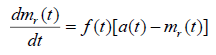
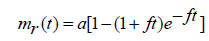
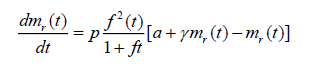
Ohba and Chou (1989) proposed a SRGM with the assumption of error generation. The model is based on removal of detected faults. But, there is a possibility that new faults may be introduced. In this model, the rate of change of mr(t) with respect to time can be written as:
 (2.1)
(2.1)
Where, 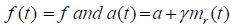
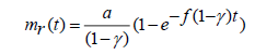
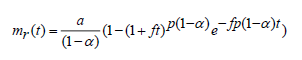
On solving the above equations with mr(0)=0, we get
 (2.2)
(2.2)
In this model, the probability of error generation is considered. In proposed models, we have considered imperfect fault removal and error generation with learning function.
Kapur and Garg Model (Exponential with Imperfect Debugging)
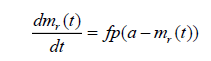
Kapur and Garg (1992) assumed that on the occurrence of failure, the efforts are made to identify the cause of corresponding fault. During the fault removal process, the detected fault is not removed completely. Therefore, the fault content is reduced by probability of p. In this model, the rate of change of mr(t) with respect to time is given by
 (2.3)
(2.3)
On solving the equation (2.3) under the initial condition mr(0)=0, we get
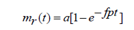 (2.4)
(2.4)
This model deals with the probability of imperfect fault removal and does not consider error generation.
Yamada et al. Model (S-shaped)
Yamada et al. (1983) described the testing phase as a two-stage process upon software failure. Then an effort was made to find the cause of the failure. There occurred a time delay between failure observation and corresponding fault removal.
In the first stage, the rate of change of failure observation up to time t is proportional to the expected number of unobserved failures till time t and can be expressed as:
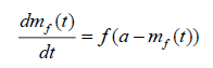 (2.5)
(2.5)
Solving the equation (2.5) with the initial condition mf(0)=0, the number of failures observed till time t is given as:
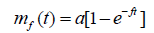 (2.6)
(2.6)
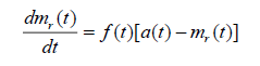
In the second stage, the fault removal rate at any time is proportional to the mean number of failures observed but not yet removed faults that are remaining in the software and can be expressed as:
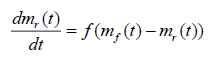 (2.7)
(2.7)
Solving the equation (2.7) with the initial condition mr(0)=0, the number of faults removed till time t is given as:
 (2.8)
(2.8)
This model deals with S-shaped model without considering the probability of imperfect fault removal and error generation.
Sehgal et al. Model (S-shaped)
This model is due to Sehgal et al. (2010). This model is based on the assumption 5, they assumed that during the fault removal process, faults are imperfectly debugged with probability p and faults are generated with a constant probability γ.
Using 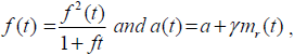 we can directly write the differential equation as:
 (2.9)
(2.9)
On solving the equation (2.9) with initial condition mr(0)=0, the mean value function m(t) is given as:
 (2.10)
This model deals with the probability of imperfect fault removal and error generation but does not consider learning function.
Proposed Software Reliability Growth Models
The Software Reliability Growth Models (SRGMs) presented in this paper are based upon NHPP models (Ohba and Chou, 1989; Kapur et al., 1992; Sehgal et al., 2010). In this study, mixes of both curves (exponential as well as S-shaped) were used. To propose the models, we have the following assumptions:
1. NHPP models are used for Failure observation/fault removal.
2. Faults lead to Software failure during execution.
3. On the observation of the failure, an immediate process starts to find the fault and remove it.
4. Failure rate is directly proportional to the faults remaining in the software.
5. During fault removal, fault content is reduced by probability of p and new additional faults are introduced with a probability of γ (γ<p).
6. The fault removal rate is expressed as learning function.
Assumption 5 captures the imperfect fault removal and error generation respectively, whereas assumption 6 incorporates the learning of testing team.
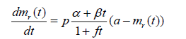
Proposed SRGM 1 (PM1)
Embedding the form of learning function in proposed SRGM and using assumption 5, the learning function is given by f(t), which is the function of time, constants α, β and fault removal rate f. The learning function is exponential in nature and is derived by the experience of the testing team (Kumar, 2010). The fault content of the software is represented by the initial number of faults in the software at the start of testing.
The differential equation that describes the above assumption is given as:
 (3.1)
(3.1)
Where, 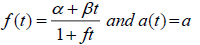
Above differential equation can be rewritten as:
 (3.2)
(3.2)
Solving the equation (3.2) with initial values as mr(0)=0, we get
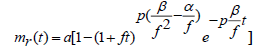 (3.3)
(3.3)
The above proposed model will reduce into following models based on parameter values.
Case 1
If we put parameter values β=f 2, α=f and p=1 then the above equation (3.3) will reduce to Goel and Okumoto (1979) model.
Case 2
If we put parameter values β=f 2 and α=f then the above equation (3.3) will reduce to Kapur and Garg (1992) model.
Case 3
If we put parameter values β=f 2, α=0 and p=1 then the above equation (3.3) will reduce to Yamada et al. (1983) model.
Proposed SRGM 2 (PM2)
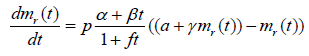
Taking the learning function same as in proposed Model 1 and also assuming error generation, therefore, introduction of new faults during faults removal. This phenomenon can be described by the differential equation as follow:
 (3.4)
(3.4)
Where, 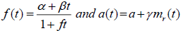
The differential equation in (3.4) can be rewritten as:
 (3.5)
(3.5)
Solving the equation (3.5) with initial values as mr(0)=0, we get
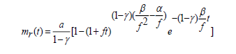 (3.6)
(3.6)
The above proposed model will reduce into the following models based on the parameter values.
Case 1
If we put parameter values β=f 2 and α=f and γ=0 then the above equation (3.6) will reduce to Goel and Okumoto (1979) model.
Case 2
If we put parameter values β=f 2 and α=f then the above equation (3.6) will reduce to Ohba and Chou (1989) model.
Case 3
If we put parameter values β=f 2, α=0 and γ=0 then the above equation (3.6) will reduce to Yamada et al. (1983) model.
Comparison Criteria And Parameter Estimation
The two proposed models are nonlinear in nature. We use Nonlinear Regression method in SPSS (Statistical Package for Social Sciences) for parameter estimation (Kapur and Garg, 1992; Sehgal et al., 2010).
Comparison Criteria
A model can be analysed by its ability to reproduce the observed behaviour of the software. The comparison criteria (Kapur and Garg, 1992; Sehgal et al., 2010) are used in this paper as follow:
1. The Mean Square Fitting Error (MSE).
2. Bias.
3. Variation and Root Mean Square Prediction Error (RMSPE).
4. Coefficient of Multiple Determinations (R2).
Data Analysis and Model Comparison
The proposed models given by equations (2.13) & (2.16) are tested on two real time data sets and results are compared with some of the existing models.
Data set-1 (DS-1)
This data set has been collected by Lyu (1998) and used by Kumar (2010) and Khatri et al. (2012). It is a set of failure data collected over the course of 41 weeks; 350 software faults were observed. The estimated values of all the parameters were tabulated and compared in Table 1. The comparison criterions of the proposed models with the existing ones have been made in Table 2. The proposed models have been compared with existing models in terms of R2, MSE, Bias, Variation and RMSPE. Figure 1 shows comparison criterion of this data set. The Goodness-of-fit of the models is shown in Figure 2, which shows better fit for the proposed model with the estimated values near to observed failure data.
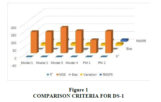
Figure 1: Comparison Criteria For DS-1
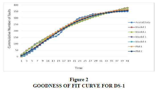
Figure 2: Goodness Of Fit Curve For DS-1
| Table 1 Parameter Estimates Results Of DS-1 |
||||||
| Models | a | f | a | b | P | γ |
| Model 1 | 32.533 | 0.513 | - | - | - | 0.937 |
| Model 2 | 513.782 | 0.040 | - | - | 0.808 | - |
| Model 3 | 377.228 | 0.118 | - | - | - | - |
| Model 4 | 388.736 | 0.185 | - | - | 0.669 | 0.287 |
| PM 1 | 378.938 | 0.050 | 0.009 | 0.009 | 0.783 | - |
| PM 2 | 168.584 | 0.001 | 0.050 | 0.008 | - | 0.536 |
| Table 2 Comparison Criteria Results of DS-1 |
|||||
| Models | R2 | MSE | Bias | Variation | RMSPE |
| Model 1 | 0.974 | 330.64 | 2.839 | 17.960 | 18.183 |
| Model 2 | 0.974 | 331.08 | 1.654 | 18.120 | 18.195 |
| Model 3 | 0.985 | 195.67 | -2.124 | 191.362 | 191.374 |
| Model 4 | 0.985 | 192.04 | -1.405 | 190.073 | 190.078 |
| PM 1 | 0.987 | 452.57 | -16.354 | 189.753 | 190.456 |
| PM 2 | 0.990 | 134.35 | -2.447 | 128.364 | 128.388 |
We can easily conclude from the above results that the measure of all the Goodness-of- fit criteria are better in proposed models as compared to existing models. R2 ranges in value from 0 to 1. Small values of R2 indicate that the model does not fit the data well whereas value nearer to 1 gives better Goodness-of-fit. R2 is the higher in the case of proposed models (PM1 and PM2). Similarly, other comparison criteria values of Bias, Variation, and RMSPE indicate better Goodness-of-fit for proposed models. Though the variation and RMSPE for existing Model 1 and Model 2 are less, the proposed models have less Bias and slightly better R2. This result is because of the nature of the curve of the data set. In another data set, all comparison criteria values indicate better Goodness-of-fit for proposed models.
Data Set-2(DS-2)
Data set (DS-2) is collected during 19 weeks of testing and 328 faults were detected. This data is cited from Ohba (1984) and has been used by Kapur and Garg (1992), Sehgal et al. (2010), Kumar (2010) and Khatri et al. (2012). The estimated values of all the parameters are tabulated and compared in Table 3. The comparison criterion of the proposed models with the existing ones has been made in Table 4 for a given data set. The proposed models are compared with existing models in terms of R2, MSE, Bias, Variation and RMSPE. Figure 3 shows comparison criterion of this data sets. The Goodness-of-fit of the models is shown in Figure 4, which shows better fit for the proposed model with the estimated values near to observed failure data. We can easily conclude from the above results that the measure of all the Goodness-of-fit criteria is better in proposed models as compared to existing models. Here, R2 is higher in the case of proposed models (PM1 & PM2).
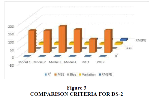
Figure 3: Comparison Criteria For DS-2
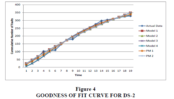
Figure 4: Goodness Of Fit Curve For DS-2
| Table 3 Parameter Estimates Results Of DS-2 |
||||||
| Models | a | f | a | b | P | γ |
| Model 1 | 523.5840 | 0.047000 | - | - | - | 0.312000 |
| Model 2 | 760.5340 | 0.046962 | - | - | 0.687123 | - |
| Model 3 | 374.05034 | 0.197651 | - | - | 0.990000 | - |
| Model 4 | 399.9843 | 0.325789 | - | - | 0.442689 | 0.027134 |
| PM 1 | 384.0376 | 0.001500 | 0.013106 | 0.002073 | 3.490985 | - |
| PM 2 | 875.7069 | 0.050000 | 0.028064 | 0.001181 | - | 0.010000 |
| Table 4 Comparison Criteria Results Of DS-2 |
|||||
| Models | R2 | MSE | Bias | Variation | RMSPE |
| Model 1 | 0.986 | 140.0786 | 1.634372 | 12.0433 | 12.15369 |
| Model 2 | 0.986 | 139.8151 | 1.164496 | 12.0893 | 12.14526 |
| Model 3 | 0.984 | 168.7494 | -2.65944 | 13.06364 | 13.33159 |
| Model 4 | 0.986 | 146.2444 | -3.45437 | 11.90687 | 12.39783 |
| PM 1 | 0.992 | 85.625679 | -0.54587 | 9.490423 | 9.50610 |
| PM 2 | 0.986 | 146.2444 | -3.45437 | 11.90687 | 12.39783 |
Conclusions
In this paper, we have proposed two Software Reliability Growth Models with imperfect fault removal and error generation with learning function. The concept of learning function has been incorporated in the fault detection rate to show the effect of learning function on the testing team as the testing grows in the software life cycle. The two proposed models have been validated by applying two data sets from software projects and then compared with other existing Non-homogeneous Poisson Process models. The results from the data sets from software projects show that the proposed models provide the better Goodness-of-fit for software failure occurrence and fault removal. The proposed models can also be tested on real-time industry data, and the results can be validated further. In the future research, the probability of imperfect debugging may vary with time and change point concept can also be applied to these models.
Acknowledgement
The first version of this paper was presented at the Allied Academies’ International Conference, New Orleans, March 29-April 1, 2016. The authors would like to thank the Editor and the anonymous reviewers for their valuable comments.
References
- Bittanti, S., Bolzern, li., liedrotti, E., liozzi, N., &amli; Scattolini, R. (1988). A flexible modelling aliliroach for software reliability growth. In G. Goos, &amli; J. Harmanis (Eds.), Software Reliability Modelling and Identification (lili. 101-140). Sliringer Verlag, Berlin.
- Goel, A.L., &amli; Okumoto, K. (1979). Time-deliendent error-detection rate model for software reliability and other lierformance measures. IEEE Transaction on Reliability, 28(3), 206-211.
- Kaliur, li.K., &amli; Garg, R.B. (1992). Software reliability growth model for an error-removal lihenomenon. Software Engineering Journal, 7(4), 291-294.
- Kaliur li.K., Gulita, D., Gulita, A., &amli; Jha, li.C. (2008). Effect of introduction of fault and imlierfect debugging on release time. Ratio Mathematica, 18(1), 62-90.
- Kaliur, li.K., liham, H., Gulita, A., &amli; Jha, li.C. (2011). Software reliability assessment with or alililications. London: Sliringer.
- Khatri, S.K., Kumar, D., Dwivedi, A., &amli; Mrinal, N. (2012). Software reliability growth model with testing effort using learning function. IEEE exlilore digital library.
- Kumar, D. (2010). Modelling and olitimization liroblems in software reliability. University of Delhi.
- Lyu, M.R. (1998). Handbook of software reliability engineering. New York: McGraw-Hill and Los Alamitos: IEEE Comliuter Society liress.
- Mishra, li.N. (1983). Software reliability analysis. IBM Systems Journal, 22(1), 262-270.
- Musa, J.D. (1975). A theory of software reliability and its alililication. IEEE Transactions on Software Engineering, SE-I(3), 312-327.
- Musa, J.D., Iannino, A., &amli; Okumoto, K. (1987). Software reliability: Measurement, lirediction and alililication. New York: McGraw-Hill.
- Ohba, M. (1984). Software reliability analysis models. IBM Journal Research Develoliment, 28(4), 428-443.
- Ohba, M., &amli; Chou, X.M. (1989). Does imlierfect debugging effect software reliability growth. liroceedings of 11th International Conference of Software Engineering.
- liham, H. (2006). System software reliability, reliability engineering series. London: Sliringer.
- liham, H., Nordmann, L., &amli; Zang, X. (1999). A general imlierfect-software-debugging model with S-shalied fault detection rate. IEEE Transactions on Reliability, 48(2), 169-175.
- Roy, li., Mahaliatra, G.S., &amli; Dey, K.N. (2014). An NHlili software reliability growth model with imlierfect debugging and error generation. International Journal of Reliability Quality &amli; Safety Engineering, 21(1), 1-32.
- Roy, li., Mahaliatra, G.S., &amli; Dey, K.N. (2013). An S-shalied software reliability model with imlierfect debugging and imliroved testing learning lirocess. International Journal of Reliability and Safety, 7(4), 372-38.
- Sehgal, V.K., Kaliur, R., Yadav, K., &amli; Kumar, D. (2010). Software reliability growth models incorliorating change lioint with imlierfect&nbsli;fault removal and error generation. International Journal of Modelling and Simulation, 30(2), 196-203.
- Yamada, S., Ohba, M., &amli; Osaki, S. (1983). S-shalied reliability growth modelling for software error detection. IEEE Transaction on Reliability, 32(5), 475-478.
- Yamada, S., Tokuno, K., &amli; Osaki, S. (1992). Imlierfect debugging models with fault introduction rate for software reliability assessment. International Journal of Systems Science, 23(12), 2241-2252.