Keywords

Turning Points, Momentum, Piecewise Linear Representation (PLR), Weighted Support Vector Machine (WSVM).

Introduction

Forecasting is broadly defined as prediction of possible future events based on past and present data. Due to its complex and dynamic nature, predicting stock market trends has been an area of interest for researchers for decades. Financial data are complex, nonlinear, nonparametric, and highly volatile. Machine learning algorithms have been successfully applied to forecasting financial data due to their success in nonlinear data analysis. Individuals tend to collect and examine information about past trends and price changes before making investments. To make a profit in the financial market, investors are more concerned with making trading decisions than forecasting daily prices (Tang et al., 2019).

A good trading policy can increase profits from investments. A Turning Point (TP) is a point at which the price of a stock changes direction. Investors like to buy or sell stocks at the TP to maximize profits. Therefore, it is crucial to accurately identify the TP of stocks.

Theoretical Framework

It is widely believed that financial markets follow a nonlinear trend (Thomaidis, 2006). For this reason, nonlinear models are used to predict stock prices and market indices.

The Efficient Market Hypothesis (EMH) was proposed in the mid-1960s (Timmermann, 2004). In an efficient capital market, stock prices reflect all available information and thus investors cannot use this information to beat the market and make significant profit (Lawrence, 1997). EMH assumes that stocks trade at their fair value and that prices rapidly adjust to new information (Hosseini Moghadam, 2004).

Various methods such as regression analysis and time series analysis have been used for forecasting. Although technical and structural analysis has been widely used in stock market prediction, evidence suggests that these methods have not been very successful. With recent advancements in this field, researchers have turned to time series models and artificial neural networks to make better forecasts (Lawrence, 1997).

Univariate time series models consider a sequence of observations of the same variable over time and use past values to predict future values (Seiler & Rom, 1997). However, although many time series are stationary, certain time series fluctuate over time (Enders, 2008).

Although statistical models have been able to provide relatively good price forecasts, the limiting assumptions inherent in some of these models undermine their effectiveness, and as a result, other methods have gradually been proposed to address these limitations and improve forecasting performance. Many studies have shown the advantages of Support Vector Machines (SVMs) and Artificial Neural Networks (ANNs) over other forecasting techniques.

Literature Review

Kara et al. (2011) compared ANN and SVM performances in predicting the direction of movement in the daily Istanbul Stock Exchange (ISE). The results indicated that the ANN model significantly outperformed the SVM model.

Huang et al. (2008) used wrapper feature selection with a composite classifier system consisting of SVM and ANN to predict stock prices. The results showed that the wrapper approach had higher prediction accuracy than the commonly used feature filters.

Zbikowski (2015) used a volume weighted SVM model with Fisher’s feature selection method to forecast short-term trends in the stock market. Seven technical indicators were used for forecasting and the results indicated the superiority of this model over plain SVM or SVM without feature selection.

Di (2014) applied SVM with technical indicators (e.g., RSI, ATR, MFI) to the prediction of stock price trends in three companies (AAPL, Amazon, and Microsoft) between 2010 and 2014. An extremely randomized tree algorithm was run on the training data with 84 features and the top features were feed into the SVM classifier. The results indicated the high degree of accuracy of the proposed method.

Luo et al. (2017) applied an improved version of the integrated piecewise linear representation and weighted support vector machine (PLR-WSVM) to 20 stocks. The results showed the success of the improved PLR-WSVM in predicting stock trading signals. They also found that the improved PLR-WSVM provides steady profits with accepted retracements.

Jadhav et al. (2018) used forecasting algorithms and ANN to predict stock market indices. Using data from BSE and NSE, they compared four algorithms (i.e., moving averages algorithm, forecasting algorithm, regression algorithm, and an ANN algorithm) and found that ANN outperformed the others. However, they argued that a combination of these algorithms can best cover possible market fluctuations and provide maximum prediction efficiency.

Shams & Parsaiyan (2012) compared the performance of Fama and French’s model to ANN in predicting stock prices in the Tehran Stock Exchange (TSE). The results indicated the superiority of the ANN model.

Fallahpour et al. (2013) used an SVM based on genetic algorithm (GA-SVM) to predict stock price movements in the TSE. GA was used to optimize the input variables of the hybrid model. The results showed that GA-SVM had a higher prediction accuracy than plain SVM.

Bajalan et al. (2017) used volume weighted SVM (VW-SVM) with F-SSFS feature selection. To forecast stock price trends. The results showed the advantage of VW-SVM model over plain SVM and the advantage of VW-SVM with F-SSFS over other conventional feature selection methods.

Mohammadi et al. (2018) proposed a hybrid model consisting of ANN and autoregressive integrated moving average (ARIMA) models for predicting changes in gold prices. The results indicated that the hybrid model outperformed plain ANN and ARIMA models.

Although various methods have been proposed to predict stock prices, the present study predicts stock turning points using PLR and WSVM in the Tehran Stock Exchange(Table 1).

Table 1 Variables And Definitions
Variable	Definition
Opening price	The first price of a security at the beginning of a trading day
High price	The highest price of a security during trading hours
Low price	The lowest price of a security during trading hours
Closing price	The price of a security at the end of a trading day

Proposed Model

Variables

Input Indices

The stock indicators are shown in Table 2 (Luo & Chen, 2013). KDJ is a composite momentum indicator that is widely used to analyze stock trends. It consists of three indicators (K, D, and J) and is calculated as follows:

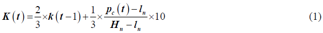
where H_n and l_nare the highest and lowest price during days.

K and D values can be set to 50 if there are no such values the previous day.

A buying signal usually occurs when K is less than D and the K line passes through the D line. When K is greater than D and the K line is below the D line, it indicates a selling signal. Therefore, different forms of KDJ are used as another input indicator.

Table 2 Indicators And Formulas
Indicator	Formula	Description
ATP		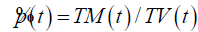Average price in a trading day
ALT		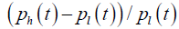Extent of price movement
ITL		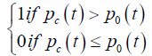K-LINE type
CATP		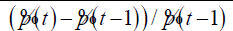Changes in average transaction price compared to the previous trading day
CTM		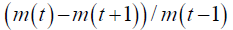Changes in transaction value compared to the previous trading day
TR		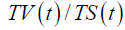Turnover rate
CTR		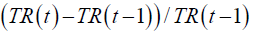Changes in turnover rate
PCCP		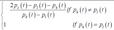Closing price position
PCTV		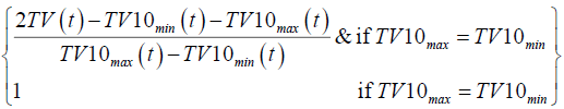Transaction volume in ten days
RDMA		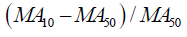Price index movement: the relative difference between two moving averages
RMACD		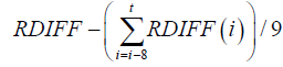Convergence/divergence of relative moving average: an indicator that follows the price trend
BASDd		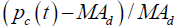Price deviation from the average
KDJ	Equations 4 to 6	Momentum indicator
ITS		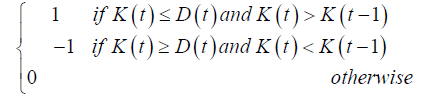KDJ type
RSId		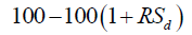The relative strength index: ratio of rise and fall in closing prices in a given period

The number of days (d) used to calculate the BIASd are 5, 10, 20, 30, and 60. The number of days (d) used to calculate the RSId are 6, 12 and 24. Overall, a total of 23 indicators are used as input variables.

Methodology

This is an applied, quantitative research and is based on field research methodology. That is, the research hypothesis is tested based on the data collected from the Tehran Stock Exchange, and then the results are generalized to the entire population.

The forecasting procedure is divided into three parts:

1. A PLR model is proposed with an unknown threshold, which can vary for different companies. In this case, the PLR threshold is selected automatically by maximizing the fitness function. 2. An oversampling method is used to determine stock TPs. The number of TPs increases if these points are treated as a period instead of a point. Random undersampling (Keogh et al., 2001) along with oversampling is used to balance the number of samples. 3. The Relative Strength Index (RSI) is used to determine whether the predicted TP is a buy point (BP) or a Sell Point (SP). 40 stocks are used to test the proposed model.

PLR, WSVM, and Zig Zag

PLR is a method for dividing a series into several segments (Luo & Chen, 2013). SVM was first proposed by Vapnik (1999) as a classification method based on structural risk minimization. SVM can provide the best generalizability with the principle of structural risk. The advantage of SVM is that it works well with small samples, nonlinear data, and high dimensional problems.

SVM transforms input vectors to a higher dimensional feature space in order to solve nonlinear problems. In that space, there is an optimal separating hyperplane that maximizes the margin between two classes. The vectors on the edges of the margin are called support vectors.

Consider the set of points is the input feature that belongs to one of the two categories according to its label A highdimensional maximum margin hyperplane is used for the nonlinearly separable problem:

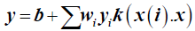
         (4)

where x is the test sample, x(i) is the support vector, and k(x (i)) is the kernel function. The kernel function can project low-dimensional variables into high dimensional variables. The polynomial kernel function 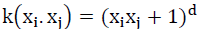and the Gaussian radial basis function (RBF) 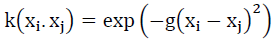are the most common alternatives.

The above equation can be converted into the following in order to obtain an optimal hyperplane:

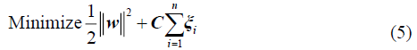
Subject to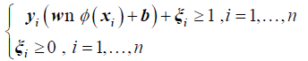

where C is the penalty factor, ξi is the slack variable, ? is the dot product, ?(xi ) is the nonlinear map, w is the vector of the hyperplane, and b denotes the bias.

When each training sample xi has a weight μi, the penalty factor C is replaced with μi c and the SVM model becomes a WSVM.

Proposed Model

The proposed model uses PLR to generate TPs and ordinary points (OPs). Weights are calculated by changes in the price of adjacent TPs. Oversampling and undersampling are used to balance the number of samples. TPs are forecast using the WSVM, and the trading signals are determined based on RSI. Figure 1 shows the flowchart of the proposed model, and the details are provided in the following subsections.

Generating TPs Using PLR

The data set is sequentially split into q training and test sets, which is calculated as follows (Zhang, 2003); (Zhong & Enke, 2017)

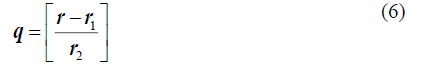
where r is the size of the data set, r1 is the size of the training set, and r2 is the size of the test set. A sample split data set is shown in Figure 2.

PLR is used in each training set to obtain stock TPs. Troughs and peaks are classified as TPs, and other points are classified as OPs.

As the number of TPs increases, PLR easily generates TPs within a short period. These points are short-term rebound points rather than TPs. Moreover, since different stocks have different price movements, it is not reasonable to set the same threshold for different stocks. The following fitness function, which focuses on medium- and long-term trends instead of short-term rebounds, can be used to solve these problems:

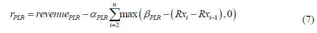
where is revenue calculated using the TPs generated by PLR, is a penalty factor, is the number of rebound points for a period where TPs should not exist, and is the day of the i th TP.

Since this equation can accurately buy at a low price and sell at a high price, the higher the number of TPs, the larger the revenue . However, the second part of the equation punishes the trades that have happened within days. The smaller the interval between trades, the greater the penalty. Therefore, the number of rebound points in PLR can be automatically determined by maximizing the fitness function .TPs and OPs are weighted differently as follows (Luo et al., 2017):

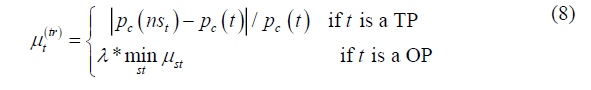
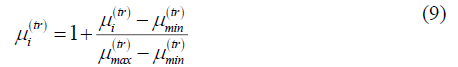
where is the closing price, is the TP, is the next TP, and is a scaled factor. Weights are normalized using the following equation:

Forecasting TPs Using WSVM

In a TP forecasting problem, TPs are labeled by financial experts or algorithms. Therefore, in the present research, a TP is treated as a period rather than a point. As such, the neighbors of TPs generated by the PLR should also be labeled as TPs, and a neighbor window is defined to control them. With the neighbor window the number of TPs increases times. Neighbors have the same weight and the same characteristics as their central TP, which makes it difficult to distinguish them. Therefore, a neighbor window is defined to control the neighbors of TPs that should not be labeled as OPs.

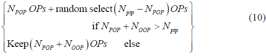
After adjusting the samples based on assuming that are respectively the number of TPs and OPs generated by PLR and is the number of other OPs, then OPs can be selected as follows:

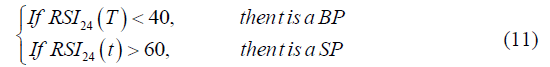
Determining Trading Signals Using RSI

After forecasting the TPs using WSVM, the next step is to determine whether these points are BPs or SPs. RSI is a technical curve based on the ratio of the sum of the number of points falling and rising in a certain period and indicates the prosperity of the stock market. The more the stock price rises, the larger the RSI, and vice versa. When RSI is around 50, the stock trend is stable, while RSI 70 and below 30 indicate overbuying and overselling, respectively (Bhargavi et al., 2017). The present research uses RSI to determine stock trends and trading signals. When stock trend is stable (i.e., RSI of around 50), it is difficult to distinguish BPs from SPs. Therefore, these points are discarded, and other points are determined as follows:

Data Analysis

The present research forecasts stock TPs using WSVM, PLR, and the Zig Zag indicator. 2019 is the target year and the period 2016-2019 is used to train the models. It must be noted that 2019 is divided into four windows, and the models are tested for each window to predict TPs and determine SPs and BPs. In addition, orders are closed at the end of each window and the profit/ loss of each window is calculated.

Iran Khodro

In this section, the TPs for Iran Khodro Automotive Company are presented. As shown in Figure 3, the WSVM-PLR algorithm generates a total of 11 TPs, 5 of which are buying signal and the rest are selling signals according to their RSI values. A total of 13 points are also obtained using the WSVM-ZigZag algorithm.

Comparing PLR and Zig Zag

Table 3 provides a comparison of profit and loss results, risk and coefficient of variation for both methods in the two modes, i.e. buying-selling positions (columns 2 and 3) and buying positions (columns 4 and 5), and the total return of each company in 2019. As can be seen, the PLR method is more efficient than the Zig Zag method in the 31 sample companies. Moreover, the risk of PLR in this case is not significantly different from Zig Zag. The coefficient of variation is also higher for PLR than Zig Zag. In columns 2 and 3 that include both buying and selling positions, these two methods are not accurate or reliable enough for forecasting. In fact, the return of these two methods has been zero compared to the total return for that year.

Table 3 Comparison Of The Performance Of Wsvm-Plr And Wsvm-Zigzag
Code	WSVM-PLR	WSVM-ZigZag	WSVM-PLR No selling	WSVM-ZigZag No selling	Total Return
IDXS	1%	-5%	33%	30%	284%
BSMZ	9%	4%	37%	26%	154%
DRZK	25%	8%	44%	30%	292%
PNBA	6%	7%	14%	8%	84%
PTEH	-13%	3%	8%	4%	130%
PRDZ	-6%	4%	16%	15%	134%
PNES	-1%	2%	12%	3%	64%
PSHZ	-1%	-5%	14%	7%	198%
MAPN	3%	-1%	19%	20%	263%
ARFZ	-1%	9%	20%	19%	87%
MKBT	5%	-4%	31%	15%	234%
PJMZ	4%	0%	17%	2%	58%
SIPA	3%	4%	22%	16%	176%
RTIR	7%	23%	47%	63%	961%
RADI	15%	19%	74%	74%	2384%
SEFH	58%	58%	125%	107%	797%
SHZG	4%	12%	35%	35%	261%
PTAP	2%	-2%	13%	10%	122%
TLIZ	24%	29%	80%	122%	662%
SBEH	-2%	-6%	24%	30%	299%
KSHJ	13%	12%	44%	41%	227%
BSDR	17%	5%	47%	7%	65%
BMLT	1%	4%	6%	6%	184%
ARNP	3%	3%	32%	24%	180%
IKHR	1%	-3%	32%	46%	392%
SAND	-5%	-7%	12%	7%	173%
BTEJ	4%	9%	19%	20%	44%
GDIR	-1%	2%	15%	12%	149%
MADN	4%	3%	14%	6%	104%
BPAR	3%	22%	65%	62%	483%
BPAS	-2%	2%	13%	25%	205%
HMRZ	-4%	2%	11%	13%	128%
PKLJ	-5%	-1%	9%	4%	226%
FKHZ	5%	1%	14%	10%	83%
SORB	-12%	4%	21%	26%	551%
FOLD	1%	-3%	10%	7%	128%
MSMI	5%	6%	29%	16%	150%
PARS	5%	2%	20%	14%	144%
PASN	1%	6%	14%	9%	114%
BARZ	11%	14%	36%	45%	318%
GOLG	-1%	1%	7%	8%	85%
CHML	0%	-2%	8%	1%	115%
KFRP	7%	4%	52%	45%	274%
NSPS	86%	83%	149%	197%	2197%
KBCZ	2%	35%	78%	72%	793%
SD	16%	16%	30%	37%	-
Mean	6%	8%	32%	30%	-
CV	262%	204%	94%	122%	-

Discussion

The Efficient Market Hypothesis (EMH) is one of the most important theories in economics and finance. On the one hand, regulators try to make the market more efficient, and on the other hand, expert traders try to profit from the difference between actual markets and an efficient market. EMH assumes that in an efficient market, all investors have access to the same information. However, many scholars and practitioners believe that price forecasts can lead to abnormal returns. To this end, various methods have been proposed for price forecasting. Machine learning and artificial neural networks are among the most widely used forecasting methods.

Conclusion

In this research, the Piecewise Linear Representation (PLR) and the weighted support vector machine (WSVM) were integrated to forecast stock Turning Points (TPs). The Relative Strength Index (RSI) was also used to distinguish between buying and selling points. By comparing PLR and Zig Zag, the results showed that both methods were not reliable when both selling and buying positions are traded. This indicates the inability of these two methods to forecast stock prices in Iran. As noted earlier, despite the upward trend and significant growth of most stocks, these methods have not been able to identify the correct ceiling and floor for entry and have had significant errors, such that their average return has been below 10 percent per year.

References

Bajalan, S., Fallahpour, S., & Dana, N. (2017). Predicting stock price trends using a modified support vector machine with hybrid feature selection. Financial Management Landscape, 17, 69-86.

Di, X. (2014). Stock trend prediction with technical indicators using SVM.Standford: Leland Stanford Junior University..

Google Scholar

Enders, W. (2008).Applied econometric time series. John Wiley & Sons..

Indexed at, Google Scholar

Fallahpour, S., Gol Arzi, G., & Faturechian, N. (2013). Predicting stock price movements in the Tehran Stock Exchange using GA-based support vector machine. Financial Research, 15(2), 269-288.    

Hosseini Moghadam, R. (2004). Market Making in the Stock Market. Jangal Publishing. 

Huang, C. J., Yang, D. X., & Chuang, Y. T. (2008). Application of wrapper approach and composite classifier to the stock trend prediction.Expert Systems with Applications,34(4), 2870-2878.

Indexed at, Google Scholar, Cross Ref

Jadhav, S., Dange, B., & Shikalgar, S. (2018). Prediction of stock market indices by artificial neural networks using forecasting algorithms. InInternational conference on intelligent computing and applications(pp. 455-464). Springer, Singapore.

Indexed at, Google Scholar

Kara, Y., Boyacioglu, M. A., & Baykan, Ö. K. (2011). Predicting direction of stock price index movement using artificial neural networks and support vector machines: The sample of the Istanbul Stock Exchange.Expert systems with Applications,38(5), 5311-5319.

Indexed at, Google Scholar, Cross Ref

Keogh, E., Chu, S., Hart, D., & Pazzani, M. (2001, November). An online algorithm for segmenting time series. InProceedings 2001 IEEE international conference on data mining(pp. 289-296). IEEE.

Indexed at, Google Scholar, Cross Ref

Lawrence, R. (1997). Using neural networks to forecast stock market prices.University of Manitoba,333, 2006-2013.

Google Scholar

Luo, L., & Chen, X. (2013). Integrating piecewise linear representation and weighted support vector machine for stock trading signal prediction.Applied Soft Computing,13(2), 806-816.

Indexed at, Google Scholar, Cross Ref

Luo, L., You, S., Xu, Y., & Peng, H. (2017). Improving the integration of piece wise linear representation and weighted support vector machine for stock trading signal prediction.Applied soft computing,56, 199-216.

Indexed at, Google Scholar, Cross Ref

Mohammadi, S., Raee, R., & Rahimi, M. R. (2018). Gold price forecasting using a hybrid ARIMA model. Journal of Financial Engineering, 9(34), 335-357.

Seiler, M., & Rom, W. (1997). A historical analysis of market efficiency: Do historical returns follow a random walk. Journal of Financial and Strategic Decisions, 10(2), 49-57.

Google Scholar

Shams, N., & Parsaiyan, S. (2012). A Comparison Between Fama And French's Model And Artificial Neural Networks In Predicting Stocks'return In Tehran Stock Exchange.  

Google Scholar

Tang, H., Dong, P., & Shi, Y. (2019). A new approach of integrating piecewise linear representation and weighted support vector machine for forecasting stock turning points.Applied Soft Computing,78, 685-696..

Indexed at, Google Scholar, Cross Ref

Thomaidis, N. S. (2006). Efficient Statistical Analysis of Financial Time-Series using Neural Networks and GARCH models.Available at SSRN 957887..

Google Scholar

Timmermann, A., & Granger, C. W. (2004). Efficient market hypothesis and forecasting.International Journal of forecasting,20(1), 15-27..

Indexed at, Google Scholar, Cross Ref

Vapnik, V. (1999).The nature of statistical learning theory. Springer science & business media.

Indexed at, Google Scholar

?bikowski, K. (2015). Using volume weighted support vector machines with walk forward testing and feature selection for the purpose of creating stock trading strategy.Expert Systems with Applications,42(4), 1797-1805.

Indexed at, Google Scholar, Cross Ref

Zhang, G. P. (2003). Time series forecasting using a hybrid ARIMA and neural network model.Neurocomputing,50, 159-175.

Indexed at, Google Scholar, Cross Ref

Zhong, X., & Enke, D. (2017). Forecasting daily stock market return using dimensionality reduction.Expert Systems with Applications,67, 126-139.

Indexed at, Google Scholar, Cross Ref

Received: 01-JuL-2022, Manuscript No. AJEE-22-12317; Editor assigned: 04-Jul -2022, PreQC No. AJEE-22-12317(PQ); Reviewed: 18-Jul-2022, QC No. AJEE-22-12317; Revised: 22-Jul-2022, Manuscript No. AJEE-22-12317(R); Published: 27-Jul -2022