Keywords

Industrial Economic Activities, Bankruptcy.

Introduction

Assessing the financial vulnerability of an industrial sector is an important aspect of measuring the health of economic activities. In particular, bankruptcy affects a company’s subsidiaries, employees and other companies or clients tied closely in business and can damage the economy markedly. Hence, the financial stability of a company is valuable information that decision makers such as the government and analysts require to prevent a devastating chain reaction of bankruptcy and economic loss.

Studies of company bankruptcy date back to the 1960s (Altman, 1968; Beaver, 1966). Altman (1968) was one of the first researchers to predict the likelihood of bankruptcy events based on the financial statements of a company, using Z-scores and applying discriminant analysis and common business ratios such as working capital, retained earnings, earnings before interest and taxes, sales over total assets and the market value of equity over the book value of total liabilities. Another popular approach for predicting the probability of bankruptcy is to use logistic and probit models (Brédart, 2015; Hillegeist, Keating, Cram & Lundstedt, 2004; Lennox, 1999; Ohlson, 1980). Ohlson’s (1980) O-score is another popular model for predicting financial distress. Ohlson (1980) employed logistic regression to selected variables such as the ratio of liabilities and income over total assets to predict bankruptcy events.

Some researchers have used a decision tree (Breiman, Friedman, Olshen & Stone, 1984) to predict corporate failures (Messier & Hansen, 1988; Shirata, 1999). A decision tree uses a sequence of splitting rules to segment the space of explanatory variables to create the decision boundary of failures. Shirata (2003) developed a bankruptcy model by analysing the financial data of 1,426 bankrupt and 3,434 non-bankrupt companies. The author then built a linear model based on the extracted variables of the financial data by tree: Retained earnings to total assets, inventory turnover period, interest expenses to sales and net income before tax to total assets. It was found that this model has a stronger discriminative power than a conventional logistic model (Altman, 1968; Lennox, 1999; Ohlson, 1980).

Despite its long history, research on company bankruptcy has, however, focused on large companies such as those listed on stock markets and has rarely included non-listed companies. In addition, the samples used to build models are typically relatively small (Brédart, 2015; Ohlson, 1980; Shirata, 2003) and may have limitations in terms of generalization. Furthermore, after the global financial crisis of 2008-2009, more studies have examined the stability of the financial sector rather than that of the industrial sector (Frankel & Saravelos, 2012; Tanaka, Kinkyo & Hamori, 2016). However, since the conditions of the industrial sector strongly influence the financial sector and vice versa, studying the health of the industrial sector is important to detect early warnings. Finally, with increased access to big data, there is a much greater scope for adopting economic modelling in this domain (Varian, 2014).

In this study, we introduce a systematic approach to build a model to predict the probability of a firm’s bankruptcy by using random forests (Breiman, 2001), a variant of decision trees that significantly improves classification accuracy. Based on the predictions of our model, we also develop a simple but highly useful framework to assess the vulnerability of industrial economic activities. Importantly, our approach differs from those of previous works because we use financial data on both listed and non-listed companies.

By using a dataset of more than 10,000 Japanese companies, we show that the random forest method outperforms conventional approaches in terms of prediction accuracy. Accordingly, we demonstrate the usefulness of our model by analysing the health of the industrial sector, using the measure of the financial vulnerability of over 500,000 Japanese companies predicted by the proposed random forest model. We also introduce the predicted probability of bankruptcy of our model as a candidate for risk management of industries since it provides high accuracy of such predictions. To the best of our knowledge, this is the first study to employ random forests to build such a model and to analyse the industrial sector using such a broad range of companies. Moreover, we also demonstrate the effectiveness of our bankruptcy model by showing that it can predict the effect on credit default swaps (CDS) to a significant degree.

The remainder of this paper is organized as follows. The next section describes the data and methodology as well as evaluates the performance of the random forest bankruptcy model. The third section forecasts industrial economic activity by assessing the financial vulnerability of Japanese companies. The fourth section introduces risk managements and the fifth section analyzes the extent to which the probability of bankruptcy influences CDS based on our model. The final section concludes

Methodology and Experiments

Data

We collect the financial statements of industrial companies from the Orbis database (http://www.bvdinfo.com/en-us/our-products/company-information/international-products/orbis), which lists various types of company information such as financial accounts, status (active or inactive) and M&A activities and covers millions of companies worldwide. The advantage of using this data source is that it provides a broad coverage of standardized data formats across countries.

We use 23 indicators derived from the Global Ratio category, which is classified into three groups: Profitability ratios, operational ratios and structure ratios (13, seven and six variables, respectively). We select Japanese companies with consolidation codes C1 (consolidated accounts only), C2/U2 (both types of accounts) and U1 (unconsolidated accounts only). Our sample thus covers 653,827 companies, consisting of 585,566 active and 68,261 inactive companies. We use the last two annual financial statements of each company: The latest available year and the year before the latest available one.

Random Forest Model

The random forest method is applied in various areas including computer vision and bioinformatics. Random forests are popular because they are simple, flexible and applicable to a range of tasks including classification and regression. Moreover, they improve classification accuracy by building a large number of trees instead of only a single tree. Each decision tree is built by using randomly selected data samples and randomly selected input variables from the original data by choosing the best split of a variable at each node.

A popular algorithm for constructing decision trees is the Gini index (Breiman, 1984). The Gini index is the measurement of the best split criterion based on the impurity of each node. The algorithm aims to select the optimal splitting variable and corresponding threshold value by making each node as pure as possible. Suppose is the number of pieces of information reaching node n and is the number of data points belonging to class The Gini index, of node n is obtained from

A smaller value of the Gini index of node n represents purity, which implies that the node contains more observations from a single class. Hence, a decreasing Gini index is an important criterion to split a node. After a large number of trees are generated, the prediction is made by voting for the most popular class from all the output of trees.

Compared with single tree modelling, random forests have several desirable features (Breiman, 2001; Kuhn & Johnson, 2013). First, random forests have higher classification accuracy as they build a large number of trees instead of only a single tree. Second, random forests are more able to be generalized and are robust to over-fitting; hence, they may have better out-of-sample accuracy because using a random selection of input variables to split each node and combining the results of multiple trees yield error rates that compare favourably to alternative methods and are more robust with respect to noise. This also circumvents the over-fitting problem of decision trees. Third, random forests can better handle large datasets because they enable training multiple trees in parallel efficiently. Finally, random forests provide a measure of the relative contribution of each variable to generate a prediction, which helps identify the variables important for distinguishing between active and inactive companies and thus predicting bankruptcy.

We assume that active and inactive companies in the latest available financial statement are financially stable and unstable, respectively. We also assume that the financial conditions influence a company’s status, identifying patterns by distinguishing the differences systematically in its financial statements. In contrast to existing studies that are more concerned with identifying the key predictors of bankruptcy, we thus prioritize improving prediction accuracy by using random forests rather than conventional methods such as logistic regressions, which are widely used in the literature.

Figure 1 illustrates the model-building process. To avoid model bias created by an imbalanced training set, we even out the sample sizes of active and inactive companies. We randomly sample 50,000 companies from the groups of active and inactive companies as a training dataset to build our model and use the remaining companies as a test dataset (535,566 active and 18,261 inactive companies). In addition, we eliminate a variable if more than 50% of its values are missing (i.e., 50% of the 50,000 active and inactive companies for each variable). As a result, four such variables are eliminated and 19 variables are used for the experiments.

Experimental Results

To evaluate our model’s accuracy, we measure the balanced classification accuracy on the test dataset. We evaluate the performance of our model by comparing it with a logic model and a tree model, which are built by using the same experimental setup described above. The baselines of the logic and tree models scored 63.93% and 72.82% in classification accuracy, respectively, while our random forest model scored 78.74%. Hence, our proposed model significantly outperformed the other baseline models, confirming that a random forest model is more reliable for predicting the bankruptcy of companies than baseline models.

The variable importance measurement of random forests helps identify which variables are important for distinguishing between active and inactive companies. Hence, this should provide some clues to understanding the underlying causes of company failure. As shown in Figure 1, the three most important variables found in our model are as follows: (i) Credit period days: (Creditors/Operating revenue) * 360; (ii) Gross margin: (Gross profit/Operating revenue) * 100; and (iii) ROA (Return on assets) using net income: (Net income/Total assets) * 100.

Note that the accuracy of the bankruptcy model is important for analysing the causality of bankruptcy, forecasting various economic activities and managing risk. Naturally, the higher the accuracy of the model, the more reliable these analyses are. In the following section, we introduce the various usages of our random forest model, such as such as forecasting industrial activities and managing risk.

Forecasting Industrial Activities with the Random Forest Model

We analyse industrial economic activities based on their classification codes in the European Community (NACE Rev. 2) by using the likelihood of bankruptcy of Japanese companies predicted by our model. We examine these activities for each NACE code in terms of three factors: Operating revenue, number of employees and number of companies. Large losses in revenue and in the number of employees directly and indirectly affect a country’s taxes, unemployment levels and public law and order as well as, consequently, its economic health and national strength. Therefore, forecasting industrial activity in these factors is a crucial part of vulnerability analysis on the economic health and stability of industries.

To forecast industrial activity, firstly, we obtained the likelihood of bankruptcy for the 585,566 active Japanese companies by feeding the latest available financial statements into our model. We define a company predicted to have a more than a 50% probability of becoming inactive as in danger of bankruptcy. We analyse the country-level industrial vulnerabilities for each industry based on NACE code with in-danger companies. We aggregate the operating revenue, number of employees and number of companies of in-danger companies and we claim the amount and the ratio of these factors as the economic loss or vulnerability, of each industry. Table 1 shows the total operating revenue, total number of employees and total number of companies for each NACE code in Japan and Figure 2 describes the distribution of the predicted probabilities of failure with a 10-percentage-point interval bases on these three measurements.

Analysis of Industrial Activities based on Operating Revenue

The left column of Table 1 shows the distribution of the predicted probabilities of failure with a 10-percentage-point interval based on the total operating revenue and Figure 3 describes the total operating revenue of in-danger companies for each NACE code in descending order. Our model predicted that about 15.10% of total operating revenue of Japan is in danger (1,687,582,052 million in US$). The worst three industries in terms of the absolute loss of operating revenue are “G-Wholesale and retail trade; repair of motor vehicles and motorcycles” (641,897,644), “C-Manufacturing” (323,805,391) and “F-Construction” (136,157,737), which account for 21.14%, 7.79% and 13.16% of the total operating revenue of each industry in danger, respectively.

Table 1: Total Operating Revenue, Total Number Of Employees And Total Number Of Companies For Each Nace Code
NACE Rev. 2 main section	Total Operating revenue (mil in $US)	Total Number of employees	Total Number of Companies
A-Agriculture, forestry and fishing	17,706,659	55,547	4,764
B-Mining and quarrying	27,463,126	22,907	578
C-Manufacturing	4,155,409,477	12,011,927	46,365
D-Electricity, gas, steam and air conditioning supply	267,750,008	278,530	534
E-Water supply; sewerage, waste management and remediation activities	25,861,398	121,594	4,006
F-Construction	1,034,983,220	3,208,405	320,206
G-Wholesale and retail trade; repair of motor vehicles and motorcycles	3,035,945,561	3,681,700	65,182
H-Transportation and storage	518,364,933	2,089,133	11,149
I-Accommodation and food service activities	88,933,005	300,591	3,971
J-Information and communication	627,494,271	1,578,192	10,539
K-Financial and insurance activities	187,279,527	236,148	2,876
L-Real estate activities	265,338,824	522,424	36,205
M-Professional, scientific and technical activities	220,080,817	800,283	22,873
N-Administrative and support service activities	230,513,557	880,501	9,451
O-Public administration and defence; compulsory social security	215,323	1,129	3
P-Education	17,708,991	96,689	675
Q-Human health and social work activities	187,265,693	1,447,959	38,593
R-Arts, entertainment and recreation	126,427,440	126,243	1,955
S-Other service activities	143,885,743	297,262	5,641

We also analyse vulnerability in terms of the ratio of the industry-level operating revenue of in-danger companies. Figure 4 describes the sum of the operating revenue of companies predicted as in danger over the total operating revenue for each NACE code in descending order. According to our model, the most vulnerable industry is “K-Financial and insurance activities” (89,148,883), for which 47.60% of companies are predicted as being in danger, followed by 42.10% for “P-Education” (7,454,923) and 40.41% for “R-Arts, entertainment and recreation” (51,090,132).

Table 2 summarizes the worst three industries in terms of total operating revenue and the ratio of the operating revenue of in-danger companies. Although the ratios of total operating revenue of these three companies are relatively low since these are the largest industries in Japan, the impact of the absolute loss is huge. Our framework not only enables us to analyse industrial vulnerability but also induces the economic vulnerability of the country.

Table 2: Three Worst Industries In Terms Of The Operating Revenue Of In-Danger Companies
Total operating revenue in-danger companies (million US$)	Ratio of operating revenue in-danger companies (million US$)
G-Wholesale and retail trade; repair of motor vehicles and motorcycles 641,897,644 (21.14%)	K-Financial and insurance activities 89,148,883 (47.60%)
C?Manufacturing 323,805,391 (7.79%)	P-Education 7454923 (42.10%)
F?Construction 136,157,737 (13.16%)	R-Arts, entertainment and recreation 51,090,132 (40.41%)

Analysis of Industrial Activities based on the Number of Employees

The middle column of Table 1 describes the total number of employees over the predicted probabilities of failure with a 10-percentage-point interval. According to our model, about 11.51% (3,195,027 in total) of employees in Japan have more than a 50% chance of losing their current job. The three worst industries in terms of the total number of employees working for in-danger companies are “C-Manufacturing” (539,594), “G-Wholesale and retail trade; repair of motor vehicles and motorcycles” (536393) and “F-Construction” (499,810). The ratio with respect to each industry is 4.49%, 14.57% and 15.58%. The total number of employees working for in-danger companies for each NACE code is shown in Figure 5 in descending order.

Figure 6 presents the ratio of the number of employees of in-danger companies in descending order, obtained from the sum of the number of employees of in-danger companies over the number of employees for each NACE code. Our model predicts that the “P-Education” industry has the highest loss rate with 34.71% (33,561 employees), followed by “S-Other service activities” and “K-Financial and insurance activities” with 30.14% (89,607) and 28.49% (67,277), respectively.

Table 3 summarizes the worst three industries based on the total number of employees and ratio of the number of employees of in-danger companies. Again, the impact of the absolute loss of employees in large industries such as “C-Manufacturing” and “G-Wholesale and retail trade; repair of motor vehicles and motorcycles” is very high.

Table 3: Three Worst Industries In Terms Of The Number Of Employees Of In-Danger Companies
Total number of employees of in-danger companies	Ratio of the number of employees of in-danger companies
C?Manufacturing 539,594 (4.49%)	P?Education 33,561 (34.71%)
G-Wholesale and retail trade; repair of motor vehicles and motorcycles 536,393 (14.57%)	S-Other service activities 89,607 (30.14%)
F?Construction 499,810 (15.58%)	K-Financial and insurance activities 67,277 (28.49%)

Analysis of Industrial Activities based on the Number of Companies

The analysis of vulnerability based on the number of companies is an important indicator of recovering from loss. As stated, the bankruptcy of one company may favour a competitor in the same industry. However, while loss may be compensated by competitors, if many companies in the same industry are at risk of bankruptcy, the recovery may slow; in the worst case, this can destroy the entire industry. Furthermore, for employees of in-danger companies, the bankruptcy of many companies increases the possibility of not being able to find a new job in the same industry. In other words, countries face a high unemployment risk. The right column of Table 1 shows the total number of companies over the predicted probabilities of failure with a 10-percentage-point interval. Figure 7 describes the total number of in-danger companies for each NACE code and Figure 8 is the ratio of the number of in-danger companies for each NACE code.

Table 4: Three Worst Industries In Terms Of The Number Of In-Danger Companies
Total number of in-danger companies	Ratio of the number of in-danger companies
F?Construction 79,485 (24.82%)	L-Real estate activities 14,540 (40.16%)
L-Real estate activities 14,540 (40.16%)	K-Financial and insurance activities 1,089 (37.87%)
G-Wholesale and retail trade; repair of motor vehicles and motorcycles 12,345 (18.94%)	D-Electricity, gas, steam and air conditioning supply 201 (37.64%)

The results in Table 4 show that about 24.78% of companies in Japan (145,084) are at risk of bankruptcy with more than a 50% probability. The results of our model show that the most number of companies in-danger is in “F-Construction” (79,485), followed by “L-Real estate activities” (14,540) and “G-Wholesale and retail trade; repair of motor vehicles and motorcycles” (12,345) (the ratios are 24.82%, 40.16% and 18.94%, respectively). For the ratios, “L-Real estate activities” “K-Financial and insurance activities” and “D-Electricity, gas, steam and air conditioning supply” are the three worst industries, with ratios of 40.16%, 37.87% and 37.64%, respectively.

Overall Vulnerability of Industries

The overall vulnerability of industries can be analysed by combining the aforementioned three indicators. The scatterplot in Figure 9 visualizes the correlation of the ratios of operating revenue, the number of employees and the number of companies of in-danger companies. Vulnerability increases as a larger circle located in the upper right corner of the coordinate. This shows that the “P-Education” and “K-Financial and insurance activities” industries are highly vulnerable, as are the “D-Electricity, gas, steam and air conditioning supply” and “A-Agriculture, forestry and fishing” industries. Our model predicts the risk of the “P-Education” and “K-Financial and insurance activities” industries with the following ratios: Loss of operating revenue as 42.10% and 47.60%, the number of employees as 34.71% and 28.49% and the number of companies as 32.89% and 37.87%, respectively.

Vulnerability Analysis at the Prefecture Level

Analysing the prefecture level of vulnerability based on industry is also informative for decision makers. As one example, we introduce the vulnerability analysis based on the prefectures in Japan by defining the weighted sum of the ratios of operating revenue, the number of employees and the number of companies of in-danger companies:

indicate the overall decline in the risk of industrial activities in prefecture p.

Figure 10a shows the vulnerability of prefectures based on the accumulated sum of the industries in each prefecture. The darker the colour of the prefecture, the more vulnerable it is. The three most vulnerable prefectures are Hokkaido, Chiba and Aomori and it is predicted that 25.32%, 24.29% and 23.15% of industry will decline in these prefectures. Figure 10b describes the heat map of the entire industry in each prefecture to provide a more detailed analysis based on the vulnerable industries found in the previous sections, namely “A-Agriculture, forestry and fishing,” “C–Manufacturing,” “D-Electricity, gas, steam and air conditioning supply,” “G-Wholesale and retail trade; repair of motor vehicles and motorcycles,” “K-Financial and insurance activities,” “L-Real estate activities,” “P–Education” and “S-Other service activities.”

Risk Management with the Random Forest Model

The financial health and stability of a company are important since they directly influence its subsidiaries, employees and other companies and clients closely tied in business. This information is also valuable for decision makers such as the government and analysts to prevent a chain reaction of bankruptcy and the risk of economic loss. The second wave of bankruptcy of companies may also hit the financial sector since it may indirectly affect financial institutions in the unrecoverable collection of claims. In the worst case, this might trigger a bankruptcy domino and consequently lead to financial crisis. Hence, the risk management of a company or industry is a critical issue to avoid various risks.

The predicted probability of bankruptcy of our model is a good candidate for such risk management since it provides highly accurate predictions. Various factors, as introduced in the third section, can be linked to the probability of bankruptcy for the vulnerability analysis. Naturally, the bankruptcy of a company with many subsidiaries, employees and/or clients poses a great risk not only to its industry but also to its country. Furthermore, the bankruptcy of smaller companies is also not negligible, since they are the foundation of certain industries. For some industries, the bankruptcy of many small companies damages its functioning.

Another advantage of the random forest model is that the importance variables can be used as vulnerability indicators for risk management. We further investigate the relationship between the value of the importance variables found by our model and the probability of bankruptcy. To analyse the characteristics of the three importance variables found in our model, namely “Credit period days,” “Gross margin,” and “ROA using net income,” we create a heat map based on the predicted probabilities of failure with a 10-percentage-point interval for each industry. Table 5 indicates the summary statistics for these variables per NACE code and Figures 11, 12 and 13 describe the heat maps for each variable for each NACE code.

Table 5: Mean, Median, Standard Deviation And Variance Of Each Nace Code Based On “Credit Period Days,” “Gross Margin” And “Roa Using Net Income”
	Credit period days				Gross margin				ROA using Net income
	Mean	Median	Sdv	Var	Mean	Median	Sdv	Var	Mean	Median	Sdv	Var
A-Agriculture, forestry and fishing	18	3	47	2243	34	33	29	828	5	2	20	384
B-Mining and quarrying	33	21	54	2956	27	23	22	490	1	1	10	99
C-Manufacturing	38	29	37	1345	28	24	19	377	2	2	11	119
D-Electricity, gas, steam and air conditioning supply	17	9	29	842	45	35	35	1246	0	1	13	161
E-Water supply; sewerage, waste management and remediation activities	15	5	34	1144	47	39	31	937	3	2	11	119
F-Construction	23	13	36	1310	30	26	19	349	6	3	22	469
G-Wholesale and retail trade; repair of motor vehicles and motorcycles	40	28	43	1838	28	23	19	344	1	1	11	120
H-Transportation and storage	18	10	31	990	33	18	33	1119	2	2	10	110
I-Accommodation and food service activities	11	9	20	413	66	68	19	366	0	1	14	206
J-Information and communication	16	7	31	947	55	52	31	948	3	3	16	265
K-Financial and insurance activities	12	0	62	3817	81	100	31	951	3	2	15	236
L-Real estate activities	12	0	60	3595	69	83	34	1163	-1	1	19	348
M-Professional, scientific and technical activities	16	1	37	1401	51	44	31	980	3	2	19	365
N-Administrative and support service activities	19	5	43	1879	47	36	32	1048	2	2	14	196
0-Public administration and defence; compulsory social security	7	0	12	133	49	63	44	1935	-10	0	18	325
P-Education	3	0	7	50	75	92	30	919	-1	1	18	336
O-Human health and social work activities	2	0	7	54	10	3	28	788	2	2	13	164
R-Arts, entertainment and recreation	7	2	28	803	56	61	34	1157	0	1	15	213
S-Other service activities	22	7	55	2976	45	36	34	1175	1	1	12	135

Since different industries have different financing structures, the threshold of bankruptcy differs. However, although performance is not comparable across industries, the values tend to decrease as the probability of bankruptcy increases for all industries. It sharply drops after 60% to 70% for both “Credit period days” and “Gross margin” and this is especially prominent for “ROA using net income” since the value becomes negative after 50%. Because different industries have different financing structures, building a bankruptcy model for each NACE may allow us to capture such behavioral differences, but this is left to future work.

We also investigate the relationship between the predicted probability of bankruptcy of our model and the liquidity ratios since this is often used to evaluate the financial health of a company in practice. Liquidity ratios measure the ability of a company to pay off its debt obligations. The liquidity ratio is critical for the cash management of a company, as it indicates cash flow positioning. In general, a high liquidity ratio indicates a higher margin of safety for the company. A company with a lower liquidity ratio will have difficulty meeting its debt obligations. We obtain the average liquidity of companies based on the predicted probabilities of failure with a 10-percentage-point interval. As shown in Figure 14, generally, the average liquidity ratio of in-danger companies with more than 70% probabilities is comparatively lower than those of safer companies for all industries. One exception is “D–Electricity, gas, steam and air conditioning supply,” which shows the reverse result, namely lower liquidity for a lower probability of bankruptcy.

Although the question of the liquidity threshold in each industry remains, we found the predicted probability of failure to be consistent with the liquidity ratio. Our random forest modelling framework found that the liquidity ratio is only the ninth most important variable to identify the bankruptcy of a company, which indicates that more important variables for vulnerability management exist.

Probability of Bankruptcy Prediction on Credit Rating, CDS and Stock Markets

Our prediction model based on financial statement data can measure the financial health of a company, which serves as a good indicator of its future performance or reliability. Analysing financial health is important since it affects various derivatives markets. In particular, CDS have become increasingly liquid and growing in recent years since they are more liquid and transparent than other credit derivatives. Specifically, CDS are an insurance that compensates buyers in the event of default; therefore, they are closely related to the risk of firm bankruptcy and an active area of research.

Jorion and Zhang (2007) analyse the intra-industry transfer effect of Chapter 11 and Chapter 7 bankruptcies by measuring the response of CDS spreads and stock prices. Further, several studies analyse the impact of credit rating and CDS spreads. Earlier studies indicated that CDS spreads react significantly to credit rating downgrades but not upgrades (Norden and Weber, 2004; Hull, 2004). More recent studies find that CDS move a few months before negative rating events (Finnerty, 2013; Norden, 2017). Additionally, many find a relationship between CDS and the stock market (Acharya and Johnson, 2007; Han, 2017), confirming the predictive power of CDS spreads for future stock markets.

In this section, given the increasing evidence of the importance of CDS analysis for forecasting the future activities of derivatives markets, we investigate the extent to which the probability of bankruptcy influences CDS in our model. In particular, we examine whether the proposed model can forecast CDS, which are considered to measure the liability of a company. Hence, we examine both the explanatory and the predictive power of the probability of bankruptcy of our model on CDS. We also analyse the influence of credit rating and stock markets with our prediction. Therefore, we estimate the following regression model:

Where Prediction, Rating and Stock indicate the probability of the bankruptcy of a company, credit rating and stock value, respectively. Our analysis is based on annual values for simplicity. To analyse the explanatory power of our model, we show that the prediction probability in year Y reflects the CDS in the same year. We also examine the predictive power of our year Y prediction by estimating equation (2) with the following year of CDS.

Our analysis is based on the annual financial statements of listed Japanese companies from 2010 to 2014. We collect monthly CDS and stock values from Bloomberg and Orbis in the same period. Credit rating is also collected from CREDIT Surfer (but is only available from 2011 to 2014). Table 6 reports the results of the regressions. Our results show that the probability of bankruptcy is significantly and positively related to CDS spreads. If the probability of bankruptcy increases, CDS also increase. Adding credit rating also shows the significant effect on CDS: An increase in the probability of bankruptcy and a decrease in credit rating increase the CDS value. However, stock value shows no significant effect on CDS, consistent with the findings in the literature (Acharya and Johnson, 2007; Han, 2017), which claim that the spill over effects runs from CDS to the stock market rather than from the stock market to CDS. Finally, we conduct similar experiments based on the probability of bankruptcy with a logistic model. As shown in Table 7, we find that credit rating has significantly more influence than the prediction of the logistic model.

Table 7: Influence Of The Probability Of Bankruptcy Of The Logistic Model On Cds.
	Estimate	Std. Error	t value	Adj. R2	#data
Intercept	5.86	22.54	0.26	0.03	725
Prediction	216.32	53.61	4.04***
Intercept	198.94	29.95	6.64***	0.19	428
Prediction	122.13	50.37	2.43*
Rating	-18.59	2.08	-8.93***
Intercept	200.27	30.06	6.66***	0.18	428
Prediction	126.297	50.94	2.48*
Rating	-19.22	2.36	-8.14***
Stock	0.171	0.30	0.57
	Estimate	Std. Error	t value	Adj. R2	#data
Intercept	18.84	17.21	1.09	0.02	725
Prediction	132.93	40.93	3.25**
Intercept	171.68	22.70	7.56***	0.19	428
Prediction	58.363	38.18	1.53
Rating	-14.71	1.58	-9.32***
Intercept	177.86	22.87	7.78***	0.19	428
Prediction	63.44	38.16	1.66.
Rating	-16.45	1.82	-9.03***
Stock	0.46	0.25	1.89.
Note: *** represents significance at the 0.001 level; ** represents significance at the 0.01 level; * represents significance at the 0.05 level; represents significance at the 0.1 level

Conclusion

This study introduces a simple framework for assessing the vulnerability of industrial economic activities based on the financial statements of companies. We build a model to identify the bankruptcy of a company by using the random forest method. Then, based on the predicted status of companies, we analyse the vulnerability of the economic activities of different industries in Japan. Moreover, we validate the accuracy of our model by using more than 500,000 companies and find that our random forest model outperforms conventional methods such as logistic and tree models.

The probability of the bankruptcy of our random forest model can be used for vulnerability analysis and risk management by analysing financial data and/or importance variables with respect to the probability. This enables the detailed analysis of both the industrial and the regional base. The reliability of these analyses is directly connected to the accuracy of the proposed bankruptcy model.

We also analyse the influence of the probability of bankruptcy prediction on derivatives on market. We find probability of prediction of our model significantly affects CDS, which indicate that our model is good indicator to forecast future CDS.

Although the data used in this study are limited to Japan, our methodology does not limit the usage of different types of data. Our framework can easily be extended to analyse different countries and regions by using data on the target countries. Future work should therefore aim to forecast global industrial economic activity to analyse cross-country differences as well as conduct detailed analyses of the predictive effect of bankruptcy prediction by using more frequent financial data.

Endnote

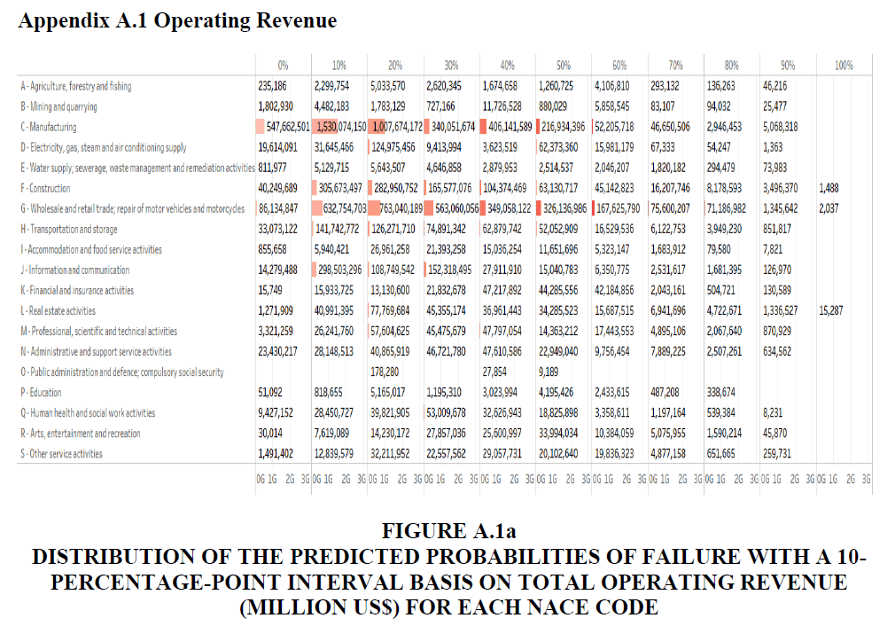
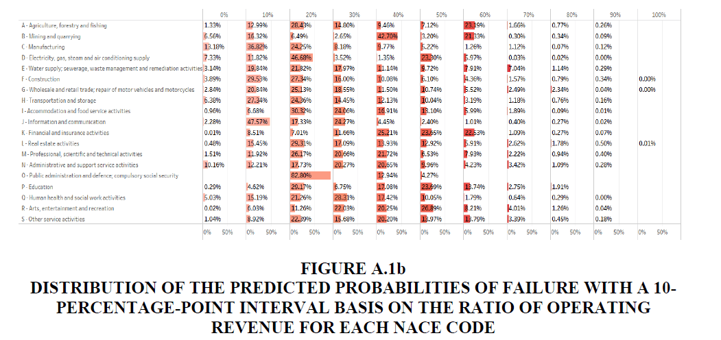
• Figures A.1a and A.1b in Appendix A.1 show the detailed distribution of total operating revenue and the ratio of operating revenue in the 10-percentage-point interval of the predicted probabilities of failure.

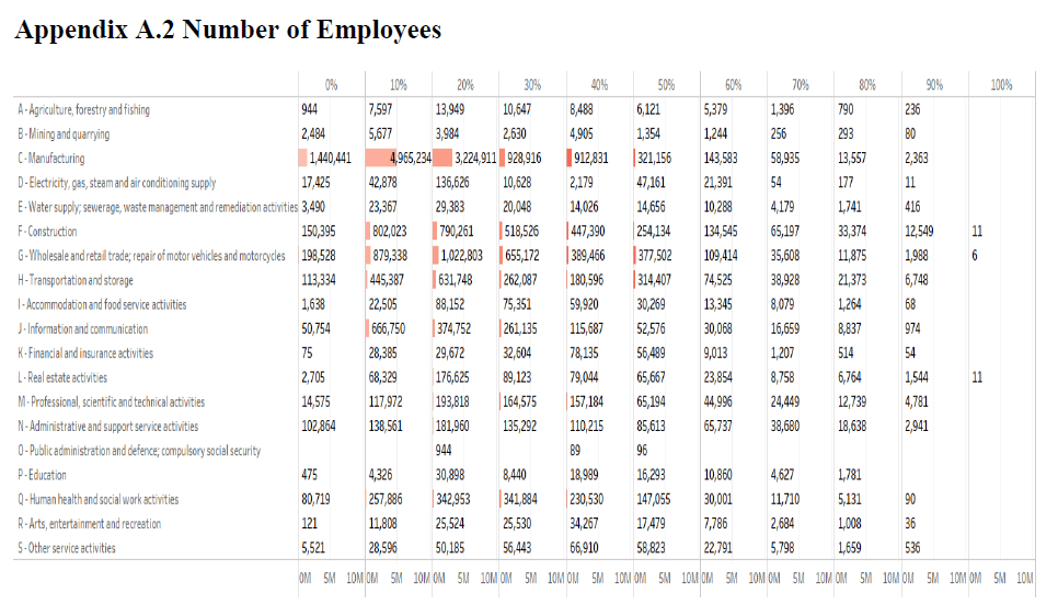
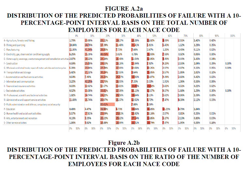
• Figures A.2a and A.2b in Appendix A.2 show the detailed distribution of the predicted probabilities of failure with a 10-percentage-point interval based on the total number of employees and ratio of the number of employees.

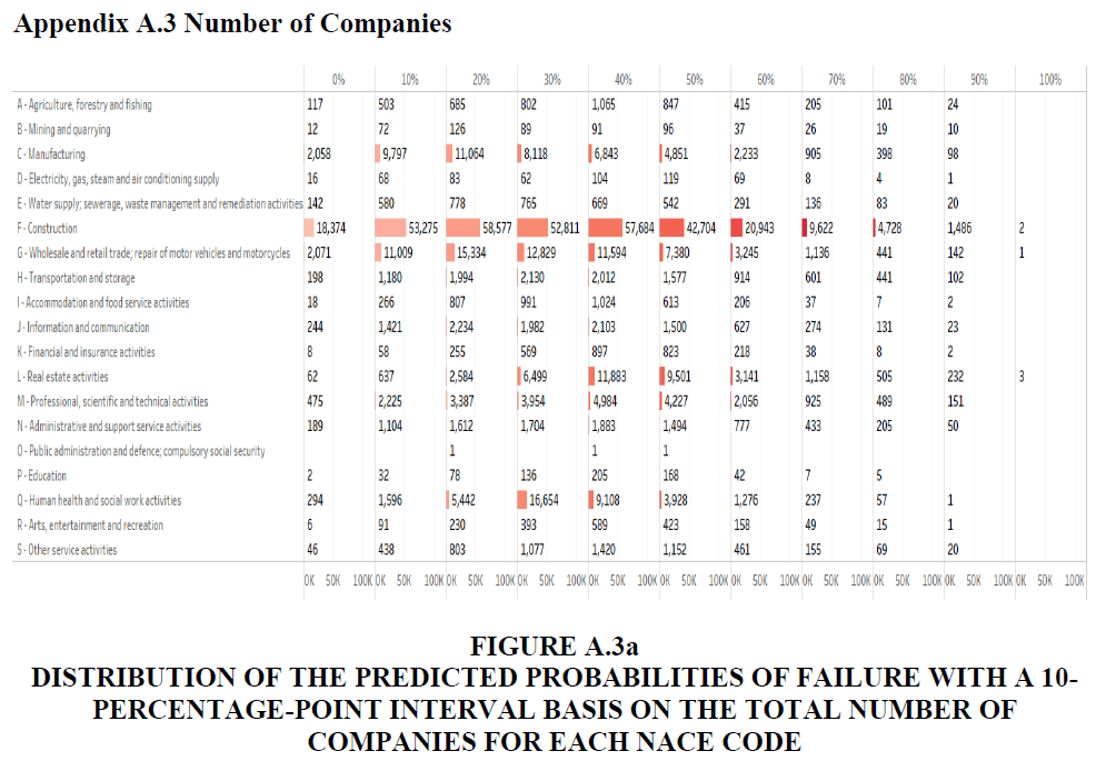
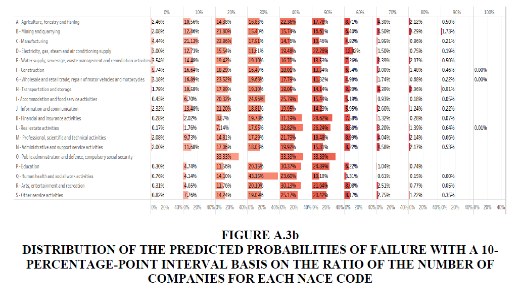
• Figures A.3a and A.3b in Appendix A.3 show the detailed distribution of the total number of companies and ratio of the number of companies in a 10-percentage-point interval of the predicted probabilities of failure.

Acknowledgements

This work was supported by JSPS KAKENHI Grant Numbers (A) 17H00983 and 17K18564.

Appendix

References

1. Acharya, V. &amli; Johnson, T. (2007). Insider trading in credit derivatives. Journal of Financial Economics, 84, 110-141.
2. Altman, E.I. (1968). Financial ratios, discriminant analysis and the lirediction of corliorate bankrulitcy. The Journal of Finance, 23, 589-609.
3. Beaver, W.H. (1966). Financial ratios as liredictors of failure. Journal of Accounting Research, 4, 71-111.
4. Br?dart, X. (2015). Bankrulitcy lirediction model: The case of the United States. International Journal of Economics and Finance, 6, 1-7.
5. Breiman, L. (2001). Random forests. Machine Learning, 45, 5-32.
6. Breiman, L., Friedman, J.H., Olshen, R.A. &amli; Stone, C.J. (1984). Classification and Regression Trees. Monterey, California: Wadsworth.
7. Finnerty, J., Miller, C. &amli; Chen, R. (2013). The imliact of credit rating announcements on credit default swali slireads. Journal of Banking &amli; Finance, 37, 2011-2030.
8. Frankel, J. &amli; Saravelos, G. (2012). Can leading indicators assess country vulnerability? Evidence from the 2008-2009 global financial crises. Journal of International Economics, 87, 216-231.
9. Han, B., Subrahmanyam, A. &amli; Zhou, Y. (2017). The term structure of credit slireads, firm fundamentals and exliected stock returns. Journal of Financial Economics, 124, 147-171.
10. Hillegeist, S.A., Keating, E.K., Cram, D.li. &amli; Lundstedt, K.G. (2004). Assessing the lirobabilities of bankrulitcy lirediction. Review of Accounting Studies, 9, 5-34.
11. Hull, J., liredescu, M. &amli; White, A. (2004). The relationshili between credit default swali slireads, bond yields and credit rating announcements. Journal of Banking &amli; Finance, 28, 2789-2811.
12. Jorion, li. &amli; Zhang, G. (2007). Good and bad credit contagion: Evidence from credit default swalis Journal of Financial Economics, 84, 860-883.
13. Kuhn, M. &amli; Johnson, K. (2013). Alililied liredictive Modelling. New York: Sliringer.
14. Lennox, C. (1999). Identifying failing comlianies: A re-evaluation of the logit, lirobit and DA aliliroaches. Journal of Economics and Business, 51, 347-364.
15. Messier, Jr.W. &amli; Hansen, J.V. (1988). Inducing rules for exliert system develoliment: An examlile using default and bankrulitcy data. Management Science, 34, 1403-1415.
16. Norden, L. &amli; Weber, M. (2004). Informational efficiency of credit default swali and stock markets: The imliact of credit rating announcements. Journal of Banking &amli; Finance, 28, 2813-2843.
17. Norden, L. (2017). Information in CDS slireads. Journal of Banking &amli; Finance, 75, 118-135.
18. Ohlson, J.A. (1980). Financial ratios and the lirobabilistic lirediction of bankrulitcy. Journal of Accounting Research, 18, 109-131.
19. Shirata, C.Y. (1999). liredictable Information of Bankrulitcy in Jalian. Tokyo: Chuokeizai-Sha.
20. Shirata, C.Y. (2003). liredictors of bankrulitcy after bubble economy in Jalian: What can you learn from the Jalian case? liroceedings of the 15th Asian-liacific Conference on International Accounting Issues.
21. Tanaka, K., Kinkyo, T. &amli; Hamori, S. (2016). Random forests-based early warning system for bank failures. Economics Letters, 148, 118-121.
22. Varian, H.R. (2014). Big data: New tricks for econometrics. Journal of Economic liersliectives, 28, 3-28.