Keywords

Stock Index, Gold, Currency Value Adjusted Index.

JEL

C43, G10, F36

Introduction

Indexes measure the overall performance of market components. These market components include combinations of firms grouped by size, industry, geography, risk and other factors. The importance of indexes cannot be overstated. Many investors follow indexes. Indeed, news organizations throughout the world report financial index levels multiple times each day. Researchers regularly use financial indexes in their studies. For example, researchers often use the Standard and Poor’s 500 index as a proxy for the market return in Capital Asset Pricing Model tests. Thus, developing indexes that provide accurate and usable information is critical.

Many methods exist to calculate indexes. Some indexes use a price-weighted approach while others use a value-weighted methodology. Some indexes include dividends, and others exclude dividends. Various other methodologies come into play in calculating indexes. Considerable debate exists regarding the appropriate currency base for asset valuation. The U.S. dollar commonly represents the basis for U.S. based asset valuation. However, in recent years, the U.S. dollar has shown considerable value variation. This variation suggests that indexes based on U.S. dollar values do not provide an accurate picture of wealth changes. Jalbert (2016, 2015a, 2015b, 2014 & 2012) proposes adjusting indexes to reflect the dollar value, relative to a basket of currencies, to provide a better measure of overall wealth changes.

While currency basket adjusted indexes represent an improvement over traditional indexes, some issues remain. Currency baskets are constructed based on a small number of currencies. For example, the Dollar Index (DXY) index compares the U.S. dollar to a basket of six currencies. These currencies may, or may not, be representative of U.S. dollar worldwide purchasing power. If the U.S. dollar is highly correlated with the basket currencies but uncorrelated with other currencies, the adjustment provides only a marginal improvement. Moreover, methodological issues used to create the currency basket further complicate their use. Given these limitations, other methods to currency value adjust indexes might provide additional insights.

Many asset valuation bases exist. Indeed, many currencies have come and gone over the history of humankind. However, gold has remained a median of value for centuries. Evidence of human desire to hold gold dates back to at least the 5th millennium BC (McKenzie, 2015). The Lydian’s first used gold as a currency in 560BC (Southerland, 1969). There exists more than 187,200 tons of mined gold (Thompson Reuters, 2016). Thus, gold provides an alternate metric for standardizing indexes. The United States departed from the Gold Standard in 1971. Since then, the dollar value of gold fluctuates based on market forces. The resulting U.S. dollar value of gold displays considerable volatility in recent years. Between January 1, 1993 and June 12, 2015, the price of gold varied from $253.90 to $1,900.60 per ounce. Alternatively, the value of one U.S. dollar has varied from 0.003952569 ounces of gold to 0.00052615 ounces of gold. This change represents approximately a 7.7 times decrease in the value of the dollar relative to gold over a 23-year period.

Some argue for a return to the gold standard. Others argue that States create alternate currencies (Ellis, 2012). Greene and Hosey (2014) discuss various Sound Money bills proposed and passed by legislatures of various U.S. states. The basic tenant behind these bills allows individuals to pay their state obligations and receive payments from the state in gold. Bitcoin provides another valuation media.

The substantial changes in U.S. dollar valuation relative to gold, as noted above, provide the motivation for this study. The appropriate value metric to examine stocks is not clear. Thus, research examining various valuation metrics positively contributes to the investment literature. This paper uses gold as a basis of valuation. While having limited usefulness as a medium of exchange, gold provides a century’s old measure of value that exceeds the existence of any known currency. We wish to know how U.S. stock indexes behave when gold is used as the underlying currency rather than the U.S. dollar. The indexes developed in this paper allow investors to easily observe how combined stock and currency changes impact their overall wealth. These combined changes will particularly interest individuals who invest in the U.S., but convert their U.S. earnings to a foreign currency for consumption. Indeed, the U.S. State Department estimates that 7.6 million U.S. citizens live abroad (U.S. State Department, Bureau of Consular Affairs, 2017). Moreover, the potential exists for development of futures and options contracts based on the indexes created in this paper. Finally, U.S. stock indexes provide the basis for many assets pricing model tests, including tests of the Capital Asset Pricing Model. The indexes developed here offer the potential for re-evaluating tests of asset pricing models.

The following analysis adjusts eight U.S. stock indexes to reflect their value in gold. We then calculate properties of these adjusted indexes. The remainder of the paper is organized as follows. The next section discusses the relevant literature. The following sections provide a discussion of the data and methodology utilized in the paper and present empirical results. The paper closes with some concluding comments and suggestions for further research.

Literature Review

A considerable literature examines the relationship between gold prices and oil prices. Hammes and Wills (2005) demonstrate the 1970’s oil shocks are not surprising given gold price changes. They show the amount of gold required to purchase a barrel of oil remained relatively constant over this period. However, the U.S. dollar value depreciated in terms of both oil and gold. Thus, the increasing dollar price of oil is not surprising. They show that one ounce of gold purchased from just less than 10 barrels of oil to 34 barrels of oil over their study timeframe. Wang and Chueh (2013) examine the relationship between interest rates, the US dollar, gold and crude prices. Their results show that oil and gold prices positively influence each other. Further, they identify a long run relationship whereby interest rates impact the U.S. dollar and the U.S. dollar subsequently influences crude oil prices.

A relatively new line of literature examines currency adjusted stock indexes. Jalbert (2016, 2015a, 2015b, 2014, 2012) argues a single currency does not provide a clear measure of value in light of currency value fluctuations. In a series of articles, he adjusts stock index levels to reflect changes in underlying currency values. He adjusts indexes to reflect the U.S. dollar value relative to a basket of currencies. His results show that annual returns calculated using original index data markedly differ from returns calculated using currency value adjusted indices. Annual, original and currency value adjusted, returns frequently have different signs, whereby, for example, the original index indicates a positive annual return and the currency adjusted index indicates a negative return. He defines total wealth change to equal the combined change in original index levels plus currency value changes. His results show that currency level changes explain as much as 8.4 and 14.9 percent of total wealth changes depending on the methodology used and time period examined.

Other researchers examine the relationship between gold prices and stock prices. Bhunia and Mukhuti (2013) examine the impact of domestic gold prices on stock price indices in India. Their results show no causality between gold prices and some stock indices. They find bidirectional causality between gold prices and other stock indices. Blose and Shieh (1995) examine the impact of gold prices on mining stock values. They find gold price elasticity exceeds one for primarily gold mining company stocks.

Many factors come into play in determining gold prices. These factors include inflation rates; political tension; jewelry and industrial demand; individual investment demand; gold production; government based purchases and sales; trade imbalances; and the state of the economy. Bauer and Lucy (2010) examine two potential roles of gold. Gold can function as a hedge against stocks or as a safe haven. They examine the relationship between stock and bond returns of three countries and gold returns. The results show that on average gold serves as a hedge against stocks. However, in extreme stock market conditions, gold serves as a safe haven. Hood and Malik (2013) find that gold provides a hedge and a weak safe haven for the U.S. stock market declines. However, they find the Volatility Index (VIX) functions as a better hedge against the stock market than gold. Choudhry & Hassan (2015) find gold does not function well as a safe haven during financial crises. However, gold functions well as a hedge against stock market return declines in less turbulent financial conditions.

Capie, Mills and Wood (2005) examine gold as a hedge against the dollar. They examine gold prices as related to sterling-dollar and yen-dollar exchange rates. They find that while gold serves as a hedge against changes in dollar value, the hedge is dependent upon unpredictable economic and political events. Joy (2011) examines dynamic conditional correlations for dollar-paired exchange rates. His examination, covering a 23 year period, shows that gold behaved as a hedge against the dollar and not as a safe haven. Lin (2012) examined co-movement between exchange rates and stock prices. He found stronger co-movements during crisis periods, thereby supporting the concept of contagion during crisis periods.

Other articles examine the extent to which gold prices conform to the cost of carry model. Blose (2010) argues the cost of carry model predicts that gold prices will not respond to expected inflation changes. His evidence shows that gold prices do not respond to unanticipated CPI changes, thereby providing support for the cost of carry model. Zhao, Chang, Su & Nian (2015) examine gold price bubbles. They identify five gold bubbles between 1973 and 2014 and argue that investor flights to safety drive these bubbles.

Indexes provide a basis for examining stock market efficiency. Kallberg & Pasquariello (2008) examine excess co-movement in stock indexes. They find co-movement, above and beyond expected, after controlling for four fundamental factors. Armano, Marchesi & Murro (2003) examine the extent that stock indexes can be forecast by a population of experts, each using genetic and neural tools. Their results indicate forecasting success that repeatedly beats a buy and hold strategy.

Data and Methodology

Data were obtained from EODdata, LLC. EODdata provides data based on a subscription model. Data were collected for the Gold index (GLD) and eight U.S. based stock indexes. The Gold index measures the value of gold in U.S. Dollars. Alternatively, the Gold index measures the value of the U.S. dollar in gold. The stock indexes include the Dow Jones Industrial Average (DJI), Dow Jones Transportation Index (DJT), Nasdaq 100 (NDX), New York Composite Index (NYA), Russell 1000 Index (RUI), Nasdaq Bank Index (BANK), MidCap 400 Index (MID) and Standard and Poor’s 500 Index (SPX). The study examines these indexes because of their popularity and data availability over the sample period. Daily data utilized in this study cover the dates December 31, 1992, through June 12, 2015. Stock index data includes 5,855 daily observations. Gold index data included 5,954 daily observations. For a time during the sample period, gold prices were reported on weekends. To synchronize the data, 99 nonmatching gold index daily observations were eliminated from the data. To further correct the sample, reported data for 211 non-trading days were removed from the sample. The resulting final dataset includes 5,644 observations.

Figure 1 shows the progression of gold prices from December 31, 1992, through June 12, 2015. Gold prices equaled $333.10 on December 31, 1992. The price of gold reached a sample period low of $253.90 on July 19, 1999. Gold prices reached a sample period high of $1,896.66 on August 11, 2011. The final data point on June 12, 2015, reveals a gold price of 1,180.93. The daily standard deviation of gold prices over the period equals 460.65.

This paper adjusts each original index to reflect values of the index in gold. Changes in these indexes represent the total wealth change of investors, including both stock value changes and currency value changes. Consider an index with level, IL_t, at time t. Consider further a gold price at time t equaling GLD_t and the base price of gold at the initiation of the adjusted index, GLDB. Then the adjusted index level at time t, AIL_t equals:

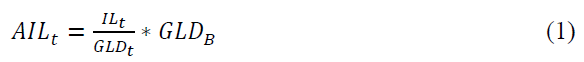
December 31, 1992, represents the index base date with a closing price of gold equal to $333.10. On this date, the original index level equals the adjusted index level.

Figure 2 graphically displays the time-series progression of each index combination. The darker line in each graph represents the unadjusted index. The lighter line indicates the adjusted index. Tables 1 and 2 shows the original and adjusted indices approximately equaling from 1993 through 1998. From 1998 through 2002, the adjusted indices generally exceeded the original indexes. From 2003 through the end of the sample period, each original index exceeded the adjusted index.

Results

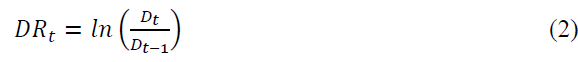
Individuals regularly examine annualized returns to evaluate portfolio performance. This paper compares original and adjusted index calendar-year-annual returns. Consider an index with level IL_t, at time t, and level IL_t-1 one year prior. The annual return, DR_t, at time t, equals the natural log of the price relatives as follows:

Annual returns for each original and adjusted series reveal substantial differences between original and adjusted index annual returns. For example, in 1997, the adjusted indexes produced a 22.91% higher return than the original indices. Similarly, in 2013, the adjusted indexes produced a 33.20% more return than the original indexes.

However, in most years the original index levels exceed the adjusted index. This finding suggests overly optimistic original indexes which may mislead investors. For example, in 2007, the original index produced a 27.49% higher annual return than the adjusted, counterpart index. Indeed, in ten of 23 years examined, original and adjusted index annual returns differed by more than 15 percent. Overall, the evidence clearly suggests relying on original indexes to measure investor wealth change can seriously mislead investors.

To further examine differences between original and adjusted indexes, the examination turns to daily index returns. Table 1 provides an analysis of daily return sign agreement. Column three shows the number of sign matching daily returns. For the Dow Jones Industrial Average, original and adjusted series daily returns had the same sign on 4,310 of 5,643 daily observations. Column 4 shows the number of daily returns with signs that disagree. For Dow Jones Industrial Average data, the paired series had opposite signs on 1,333 observations. Column 5 shows the percentage of daily returns with sign agreement. For the Dow Jones Industrial Average, the original and adjusted indices agreed on 76.38 percent of observations. The series disagreed regarding sign on 23.62 (100-76.38) percent of the data points. The remaining series produce similar results with agreement percentages ranging from 68.16% to 81.59%.

Table 1: Daily Change Analysis
Index	Observations	Sign Agreement	Sign Disagreement	Percentage Agreement
Dow Jones Industrial	5,643	4310	1,333	76.38
Dow Jones Transportation	5,643	4,571	1,072	81.00
Nasdaq 100	5,643	4,604	1,039	81.59
NYSE Composite	5,643	4,221	1,422	74.80
Russell 1000	5,643	4,311	1,332	76.40
Nasdaq Bank	5,643	3,887	1,756	68.88
MidCap 400	5,643	3,846	1,797	68.16
S&P 500	5,643	4,139	1,504	73.35

This table shows daily return statistics. Sign Agreement indicates the number of daily observations when the original and adjusted indices both have positive, or both have negative returns. Sign Disagreement equals the number of daily observations where the original and adjusted daily returns have opposite signs. Percentage Agreement indicates the percentage of daily observations where original and adjusted indexes have equal signs.

Next, the analysis examines index variance. The process of gold price adjusting indexes might exacerbate or smooth index level or return volatility. Table 2 presents a variance analysis of index levels.

Table 2: Variance Analysis For Index Levels
Panel A: Daily Data
Index	Nobs.	Original Mean	Original STD	Original Coefficient of Variation	Adjusted Mean	Adjusted STD	Adjusted Coefficient of Variation
Dow Jones Industrial	5,644	9,981.94	3,509.11	0.3515	6,365.00	3,370.59	0.5296
Dow Jones Transportation	5,644	3,746.72	1,757.82	0.4692	2,193.62	863.37	0.3936
Nasdaq 100	5,644	1,776.59	1,017.94	0.5730	1,111.25	916.49	0.8247
NYSE Composite	5,644	6,580.22	2,263.45	0.3440	4,173.41	2,089.40	0.5006
Russell 1000	5,644	615.63	219.94	0.3572	397.68	221.91	0.5580
Nasdaq Bank	5,644	1,985.33	745.85	0.3757	1,342.53	794.17	0.5915
MidCap 400	5,644	619.91	347.08	0.5599	344.15	146.22	0.4249
S&P 500	5,644	1,138.65	391.60	0.3439	744.29	426.43	0.5729
Gold	5,644	683.88	460.65
Panel B: Annual Data
Index	Nobs.	Original Mean	Original STD	Coefficient of Variation	Adjusted Mean	Adjusted STD	Coefficient of Variation
Dow Jones Industrial	24	10,572.10	3,828.71	0.3621	6,396.07	3,372.73	0.5273
Dow Jones Transportation	24	4,038.97	2,023.52	0.5010	2,232.70	865.72	0.3877
Nasdaq 100	24	1,944.53	1,150.62	0.5917	1,145.17	910.15	0.7948
NYSE Composite	24	6,922.56	2,385.36	0.3446	4,187.16	2,119.91	0.5063
Russell 1000	24	653.67	244.44	0.3740	400.16	222.92	0.5571
Nasdaq Bank	24	1,088.19	761.40	0.3646	1,347.98	801.71	0.5948
MidCap 400	24	673.24	389.19	0.5781	354.61	146.94	0.4144
S&P 500	24	1,205.29	432.81	0.3591	747.14	429.12	0.5743
Gold	24	709.36	462.15	0.6515

This table provides variance analysis for index levels. The column labeled Nobs show the number of observations in the sample. The Original Mean and Original STD columns indicate the mean and standard deviation for the unadjusted indexes. The Original Coefficient of Variation equals the Coefficient for the unadjusted series. The column. Adjusted Mean, Adjusted STD and Adjusted Coefficient of Variation indicate values for the gold price adjusted series.

Panel A and B show variance analysis of daily and annual index levels respectively. The column titled Original Mean and Original STD indicate the mean and standard deviation of unadjusted index levels respectively. The original Dow Jones Industrial Average had mean of 9,981.94 and standard deviation of 3509.11 over the sample period.

As the means are substantially different for the various indexes, for direct comparison, we calculate the coefficient of variation for each index. The Dow Jones Industrial Average results reveal a coefficient of variation equal to 0.3515. The adjusted Dow Jones Industrial Average mean equals 6,365, and standard deviation equals 3,370.59, producing a coefficient of variation of 0.5296. Thus, the adjusted series carries more than 1.5 times the amount of standard deviation per unit of return. The adjusted index coefficient of variation is higher than the original index coefficient of variation for six of eight indexes. The results in Panel B, for annual data, reveal similar characteristics. The data clearly indicates that original index levels underestimate total wealth variance.

Table 3: Variance Analysis For Index Returns
Panel A: Daily Data
Index	Nobs.	Original Mean	Original STD	Original Coefficient of Variation	Adjusted Mean	Adjusted STD	Adjusted Coefficient of Variation
Dow Jones Industrial	5,643	0.02996	1.1072	36.9597	0.00753	1.5674	208.184
Dow Jones Transportation	5,643	0.03118	1.4871	47.7014	0.00875	1.8631	213.001
Nasdaq 100	5,643	0.04457	1.1806	40.6273	0.02214	2.1297	96.200
NYSE Composite	5,643	0.02599	1.1443	44.0256	0.00356	1.5440	433.355
Russell 1000	5,643	0.02856	1.2724	44.5543	0.00613	1.6735	273.014
Nasdaq Bank	5,643	0.02987	1.3347	44.6861	0.00617	1.6056	260.195
MidCap 400	5,643	0.03996	1.2728	31.8520	0.00744	1.7476	234.885
S&P 500	5,643	0.02782	1.1702	44.0611	0.01753	1.6526	94.256
Gold	5,343	0.02243	1.0567	47.1160
Panel B: Annual Data
Index	Nobs.	Original Mean	Original STD	Original Coefficient of Variation	Adjusted Mean	Adjusted STD	Adjusted Coefficient of Variation
Dow Jones Industrial	23	7.3499	15.7833	2.1474	1.8472	23.4161	12.6764
Dow Jones Transportation	23	7.6487	17.3894	2.2735	2.1461	25.0005	11.6494
Nasdaq 100	23	10.9343	32.6339	2.9845	5.4316	36.7948	6.7741
NYSE Composite	23	6.3768	17.7766	2.7877	0.8741	24.4444	27.9639
Russell 1000	23	7.0065	18.6125	2.6564	1.5039	25.8124	17.1640
Nasdaq Bank	23	7.3281	19.8069	2.7029	1.8254	30.0606	16.4680
MidCap 400	23	9.8043	17.0405	1.7381	4.3017	23.9021	5.5565
S&P 500	23	6.8257	18.4851	2.7082	1.3230	25.8731	19.5562
Gold	23	5.5027	15.2125	2.7646

This table provides variance analysis for index returns. The column labeled Nobs indicates the number of observations in the sample. The Original Mean and Original STD columns indicate the mean and standard deviation for the unadjusted indexes. The Original Coefficient of Variation equals the coefficient for the unadjusted series. The column, Adjusted Mean, Adjusted STD and Adjusted Coefficient of Variation indicate values for the gold price adjusted series.

While index levels provide notable results, index returns also provide interesting insights. Table 3 shows variance analysis for index returns. Panels A and B provide results based on daily and annual data respectively. Daily data reveals an average daily return of 0.02996 percent and standard deviation of 1.1072 for the Dow Jones Industrial Average combining to result in a 36.9597 coefficient of variation. The corresponding adjusted index has mean of 0.00723 percent and standard deviation of 1.5674 implying a coefficient of variation of 208.18. The coefficient of variation for the adjusted series is more than five times larger than for the corresponding original series. These results indicate that original index data underestimates the level of wealth risk by a considerable margin. This phenomenon holds for each of the eight index pairs. Panel B shows similar results for the annual data analysis.

Table 4: Return Distribution Statistics
Panel A: Original Index Distribution
Index	Mean		Std. Dev.		Skewness		Kurtosis		Normality
DJI	0.02996		1.1072		-0.16759		8.3988		14.4622***
DJT	0.0312		1.4871		-0.3667		6.0187		7.7439***
NDX	0.0446		1.8106		0.0773		5.6367		14.4141***
NYA	0.0260		1.1442		-0.3939		10.7664		19.4771***
RUI	0.0286		1.2723		-0.4282		11.1843		23.4079***
BANK	0.0299		1.3347		-0.1608		12.3234		25.5233***
MID	0.0400		1.2728		-0.4015		7.2494		13.3887***
SPX	0.0279		1.1716		-0.2495		8.7375		16.7400***
Panel B: Gold Value Adjusted Index Distribution
Index	Mean	Std. Dev.		Skewness		Kurtosis		Normality
DJI	0.0075	1.5674		-0.2978		6.58934008		9.5017***
DJT	0.0087	1.8631		-0.4493		7.12434974		7.1313***
NDX	0.0221	2.1297		-0.0065		4.48611608		8.2672***
NYA	0.0036	1.5440		-0.3708		8.09126583		12.6954***
RUI	0.0061	1.6734		-0.4133		7.63067928		13.0505***
BANK	0.0074	1.7475		-0.2607		8.84535139		16.3950***
MID	0.0175	1.6526		-0.3444		6.43295247		10.3867***
SPX	0.0054	1.6034		-0.2861		6.6215983		10.2248***

The examination continues with correlation analysis. The correlations between index levels range from -0.1120 for the Dow Jones Transportation index to 0.4829 for the Nasdaq Bank index. Significant correlations occur for seven of the eight indexes. An examination of daily index changes indicate correlations range from 0.0324 for the Russell 1000 index to 0.8758 for the Nasdaq 100 index. The fourth column shows correlations between returns. The lowest return correlation occurs for the New York Composite Index at 0.7292. The highest return correlation occurs for the Nasdaq 100 at 0.8684. Each of the eight correlations is significant.

Index levels and gold prices produce significant correlations for each index. The correlations range from 0.1159 to 0.7819. Index change and gold price change results show less significance. The change correlations range from -0.0022 to 0.0673, with significance for only three of eight correlations. Five of the eight indexes show significant results for original index returns and gold returns, with correlations between -0.0553 to 0.0174. Six of seven indexes show a negative correlation.

The analysis continues with an examination of return distribution statistics. Table 4 shows results for returns. Panel A presents original index results. Panel B provides results for the Gold Value Adjusted indexes. The results reveal negative skewness for seven of eight original index distributions and for all of the Gold Value Adjusted indexes. The exception is the original NDX index. Each normality test indicates rejection of the normal distribution. Research elsewhere documents index return deviations from a normal distribution. The results here confirm that currency value adjusting indexes does not transform the series into normal distributions.

Table 5: Return Distribution Difference Tests
	T-Test	F-Test	Kolmogrov-Smirnov Test
DJI	-0.88	2.00***	4.6971***
DJT	-0.71	1.57***	2.9745***
NDX	-0.60	1.38***	2.9745***
NYA	-0.88	1.82***	4.2359***
RUI	-0.80	1.73***	4.3582***
BANK	-0.77	1.71***	3.9347***
MID	-0.81	1.69***	3.5487***
SPX	-0.85	1.88***	4.4335***

This table shows the results of distribution difference tests. The T-tests identifies difference in means. The F-test detects differences in variance. The Kolmogrov-Smirnov test identifies overall distribution differences. DJI indicates the Dow Jones Industrial Average Index. DJT indicates the Do Jones Transportation Index, NDX indicates the NASDAQ 100 index. NYA indicates the NYSE Composite index. RUI indicates the Russell 1000 index. BANK indicates the NASDAQ Bank Index. MID indicates the MidCap 400 Index. SPX indicates the Standard and Poor’s 500 Index.

Further examination of return distribution differences, involves conducting three tests of distribution equality. Table 5 provides the results. Each index fails to reject the null hypotheses of no difference in means between each original and gold value index pair. However, the F-test for equality of variances indicates significant variation differences between original and gold value adjusted indexes. Finally, the analysis uses the Kolmogrov-Smirnov to detect overall distribution differences. The results indicate rejection of distribution equality for all eight index pairs. Overall, the results here indicate that original and gold value adjusted indexes, while having the same means, do not have the same overall distribution characteristics.

To further understand relationships in the data, we conduct regression analysis. The first examination looks at index levels. The methodology includes three regressions on adjusted index levels as follows:

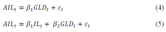
Equation 3 regresses adjusted index levels on the original index levels. Equation 4 regresses adjusted index levels on gold prices. Equation 5 regresses adjusted index levels on both original index levels and gold prices. Of interest is the extent to which each independent variable explains variance in the adjusted index level. Intercept terms are suppressed to examine the relationships between the variables directly.

Table 6 shows the results. Panel A shows the Equation 3 estimates. The results reveal the regression coefficients significantly differ from zero. This significance is not surprising, given the model construction. The analysis turns to the regression coefficient values and R2 statistics which are the primary variables of interest. The results reveal that regression coefficients range between 0.4338 and 0.6562. The R2 values range from 0.6654 to 0.7960 indicating that original index levels explain as much as 79.6 percent of adjusted index level variation. Thus, there remains substantial unexplained variance. This suggests that gold price levels represent an important component of overall wealth levels.

Table 6: Index Level Regressions
Dependent Variable	Original Index Coefficient	T	Gold Price Coefficient	T	R2
Panel A: Adjusted Index Levels versus Original Index Levels
DJI-A	0.5717	116.24***			0.7054
DJT-A	0.4699	109.67***			0.6806
NDX-A	0.5738	105.92***			0.6654
NYA-A	0.5669	118.82***			0.7144
RUI-A	0.5859	116.81***			0.7074
BANK-A	0.6562	148.39***			0.7960
MID-A	0.4338	109.37***			0.6795
SPX-A	0.6020	118.75***			0.7142
Panel B: Adjusted Index Levels versus Gold Prices
DJI-A			4.8908	50.76***	0.3135
DJT-A			1.8358	62.92***	0.4123
NDX-A			0.8705	43.17***	0.2483
NYA-A			3.2241	52.06***	0.3244
RUI-A			0.3016	48.97***	0.2983
BANK-A			0.9727	45.04***	0.2644
MID-A			0.3073	67.75***	0.4486
SPX-A			0.5579	47.73***	0.2876
Panel C: Adjusted Index Levels versus Original Index Levels and Gold Prices
DJI-A	1.1798	180.13***	-8.6948	-103.46***	0.8983
DJT-A	0.9365	100.53***	-2.5245	-53.99***	0.7894
NDX-A	1.1051	149.69***	-1.5168	-82.73***	0.8488
NYA-A	1.1308	170.31***	-5.3169	-94.89***	0.8900
RUI-A	1.1526	174.08***	-0.5074	-96.67***	0.8899
BANK-A	0.9797	195.57***	-1.0412	-80.81***	0.9054
MID-A	0.8494	87.47***	-0.3821	-45.66***	0.7660
SPX-A	1.1657	185.64***	-0.9373	-102.21***	0.8998

This table shows results of index level regressions. Panel A shows results of regressions of original index levels on adjusted index levels. Panel B shows results of regressions of gold prices on adjusted index levels. Panel C shows results of regressions of original index levels and gold prices on adjusted index levels. *** indicates significance at the 1 percent level.

Table 6, Panel B shows results of Equation 4 estimates. Each coefficient significantly differs from zero and the regression R2 statistics range from 0.2644 to 0.4486. The results indicate gold price levels explain between 26 and 45 percent of adjusted index levels. Panel C shows estimates incorporating both explanatory variables. In each regression, both the original index and gold price coefficients significantly differ from zero. R2 statistics vary from 0.7660 to 0.8998. The remaining, unexplained variance is due to correlation effects between gold price levels and original index levels.

The analysis continues by conducting regressions on index level changes. Equations 6, 7 and 8 indicate the regression specifications.

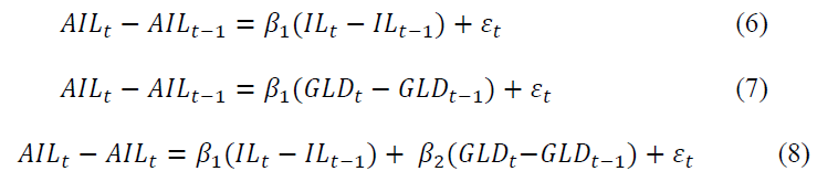
Table 7 presents the Equations 6, 7 and 8 regression estimates. Equation 6 regresses adjusted index level changes on original index level changes. The Panel A results shows that each original index coefficient significantly explains the adjusted index change. The R2 statistics range from 0.0016 to 0.7669. Equation 7 regresses gold price changes on adjusted index changes. Panel B shows significance for seven of eight regression coefficients and R2 statistics as high as 0.1880. Panel C, shows Equation 8 estimates. The results reveal that each original index return is significant in explaining adjusted index returns. With the exception of the Russell 1000 index, all gold return coefficients are also significant. R2 statistics range from 0.0017 to 0.7993.

Table 7: Index Change Regressions
Dependent Variable	Original Index Coefficient	T	Gold Price Coefficient	T	R2
Panel A: Adjusted Index Level Changes versus Original Index Level Changes
CDJI-A	0.6627	64.89***			0.4474
CDJT-A	0.5141	71.54***			0.4757
CNDX-A	0.9698	136.25***			0.7669
CNYA-A	0.5267	55.74***			0.3551
CRUI-A	1.9418	3.04***			0.0016
CBANK-A	0.5488	63.15***			0.4141
CMID-A	0.4482	59.18***			0.3830
CSPX-A	0.6778	67.04***			0.4434
Panel B: Adjusted Index Level Changes versus Gold Price Changes
CDJI-A			-4.4072	-30.97***	0.1453
CDJT-A			-1.6986	-31.63***	0.1506
CNDX-A			-0.7744	-13.60***	0.0317
CNYA-A			-2.6998	-31.59***	0.1503
CRUI-A			0.2335	0.46	0.0000
CBANK-A			-0.9077	-30.81***	0.1441
CMID-A			-0.2679	-36.14***	0.1880
CSPX-A			-0.4871	-28.07***	0.1225
Panel C: Adjusted Index Level Changes versus Original Index Level Changes and Gold Price Changes
CDJI-A	0.6620	74.95***	-4.3934	-43.61***	0.5717
CDJT-A	0.5093	82.92***	-1.6469	-45.67***	0.6172
CNDX-A	0.9702	146.89***	-0.7822	-30.17***	0.7993
CNYA-A	0.5524	68.98***	-2.9942	-47.45***	0.5391
CRUI-A	1.9383	3.03***	0.2139	0.42	0.0017
CBANK-A	0.5354	69.25***	-0.8405	-38.77***	0.5374
CMID-A	0.4606	74.74***	-0.2827	-53.76***	0.5920
CSPX-A	0.6806	76.54***	-0.4942	-40.66***	0.5696

This table shows results of index change regressions. Panel A shows results of regressions of original index changes on adjusted index changes. Panel B shows results of regressions of gold price changes on adjusted index changes. Panel C shows results of regressions of original index changes and gold price changes on adjusted index changes. *** indicates significance at the 1 percent level

Finally, we estimate index return regressions. Equation 9 and 10 specify the estimated regression equations:

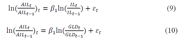
Equation 9 regresses adjusted index returns on original index returns. Equation 10 regresses adjusted index returns on gold returns. The careful reader will notice that multiple regressions were estimated for the level and change analysis. However, the return analysis includes only single regressions. The methodology used to create the variables, causes multiple regressions on the returns to result in linear combinations which cannot be estimated using ordinary least squares regression. Table 8 shows the results. Panel A shows estimation results of Equation 9. The results indicate significance for each coefficient at the one percent level. R2 statistics range from 0.5315 to 0.7540, showing the original index explains as little as 53.15 percent of changes in total returns. Panel B shows results of Equation 10 estimates. The results show significant coefficients for each regression. R2 statistics range in value from 0.2778 to 0.5018 indicating that gold returns explain as much as 50.18% of total wealth changes.

Table 8: Index Return Regressions
Dependent Variable	Original Index Coefficient	T	Gold Price Coefficient	T	R2
Panel A: Adjusted Index Returns versus Original Index Returns
CDJI-A	1.0460	82.43***			0.5463
CDJT-A	1.0320	109.20***			0.6788
CNDX-A	1.0211	131.52***			0.7540
CNYA-A	0.9835	80.01***			0.5315
CRUI-A	1.0196	92.24***			0.6013
CBANK-A	1.0434	99.14***			0.6353
CMID-A	0.9977	90.29***			0.5910
CSPX-A	1.0306	85.77***			0.5660
Panel B: Adjusted Index Returns versus Gold Price Returns
CDJI-A			-1.0505	-75.39***	0.5018
CDJT-A			-1.0635	-56.82***	0.3640
CNDX-A			-1.0621	-46.59***	0.2778
CNYA-A			-0.9806	-68.03***	0.4506
CRUI-A			-1.0285	-64.17***	0.4219
CBANK-A			-1.0692	-63.68***	0.4182
CMID-A			-0.9966	-62.13***	0.4036
CSPX-A			-1.0375	-70.41***	0.4676

This table shows results of index return regressions. Panel A shows results of regressions of original index returns on adjusted index returns. Panel B shows results of regressions of gold price returns on adjusted index returns. *** indicates significance at the 1 percent level.

Concluding Comments

Changing currency values confound stock index usefulness. Recent literature adjusts U.S. stock indexes by controlling for the U.S. dollar value relative to foreign currency baskets. This paper also adjusts U.S. stock indexes for relative values. The adjustment mechanism here involved adjusting stock indexes to reflect their value in gold. Gold provides a value metric that has stood the test of time and is universally valued. As such, it provides a stable basis for valuation. The paper examines eight U.S. stock indexes and compares them to their gold value adjusted counterparts.

The analysis examines data from January 1993 through June 2015. The results show that currency value adjusted indexes generally track at levels below the original stock index. An examination of daily index returns indicates the return signs agree on 68.16 to 82.59 percent of trading days and disagree on 17.41 to 31.84 percent of trading days. Variance analysis reveals that adjusted indexes have substantially higher variance than their original counterparts. In some instances, the coefficient of variation levels for the adjusted index equals more than five times their original index counterpart. Further testing reveals significant distribution difference for each original and gold value adjusted index pair. These findings are particularly important for tests of asset pricing models that rely on index values to measure market returns and risks.

Regression analysis shows that original indexes explain between 67 and 80 percent of adjusted index levels. Gold prices levels explain between 25 and 45 percent of adjusted index levels. Another set of regression examines index returns. The results show that original index returns explain between 53 and 75 percent of adjusted index returns while gold returns explain between 28 and 50 percent of adjusted index returns. The results here suggest that currency value changes explain a larger portion of wealth changes than found in earlier papers. For example, Jalbert (2012) and Jalbert (2014) results show that currency returns explained as much as 8.4 and 15 percent of adjusted returns respectively.

This paper is subject to some limitations. The analysis does not segregate the data into subperiods. Structural changes over time could affect the relationships examined in this paper. For example, Quantitative easing increased the supply of U.S. dollars while the quantity of gold in the market remained relatively constant. Future research might segregate the data by various regimes to identify the impact of these factors on the indexes and index distribution.

Future research might incorporate inflation levels into the modified index. While desirable, such an approach would be limited by the frequency of inflation data observations. As inflation data is generally presented monthly, such an index would be limited to monthly observations and would not be suitable for developing daily or intraday index observations. inflation data is generally presented monthly, such an index would be limited to monthly observations and would not be suitable for developing daily or intraday index observations.

Future research might also utilize other index calculation and statistical techniques to determine the robustness of results reported in this paper. Also of interest is determining more specifically which distribution family the adjusted indexes follow. From these tests additional insights might be obtained, including identifying the extent to which economic shocks result in fat-tailed distributions. A particularly interesting issue is the extent to which gold value adjusting the indexes exacerbates or placates any identified fat-tails.

This paper analyzes only U.S. indexes. Future research might examine indexes from other countries. Further, utilizing close of day data in this paper limits the analysis. Examinations of intraday data would provide additional insights. Finally, future research might examine statistical properties of the indexes in more detail.

References

1. Armano, G., Marchesi, M. & Murru, A. (2005). A hybrid genetic-neural architecture for stock indexes forecasting. Information Sciences, 170(1), 3-33.
2. Baur, D.G. & Lucey, B.M. (2010). Is gold a hedge or a safe haven? An analysis of stocks, bonds and gold. The Financial Review, 45(2), 217-229.
3. Bhunia, A. & Mukhuti, S. (2013). The impact of domestic gold price on stock price indices - An empirical study of Indian stock exchanges. Universal Journal of Marketing and Business Research, 2(2, May), 35-43.
4. Blose, L.E. & Shieh, J.C.P. (1995). The impact of gold price on the value of gold mining stock. Review of Financial Economics, 4(2), 125-139.
5. Blose, L.E. (2010). Gold prices, cost of carry and expected inflation. Journal of Economics and Business, 62(1), 35-47.
6. Capie F., Mills, T.C. & Wood, G. (2005). Gold as a hedge against the dollar. International Financial Markets Institutions & Money, 15(4, October), 343-352.
7. Choudhry, T. & Hassan, S.S. (2015). Relationship between gold and stock markets during the global financial crisis: Evidence from non-linear causality tests. International Review of Financial Analysis. 41(October), 247-256.
8. Ellis, B. (2012). States seek currencies made of silver and gold. CNN Money, February 3, downloaded June 16, 2015 from: http://money.cnn.com/2012/02/03/pf/states_currencies/
9. EODData LLC. (2015). Data downloaded from http://www.eoddata.com on June 12.
10. Greene W.L. & Hosey, N. Digging for gold: A multivariate analysis of the passage of state “Sound Money Laws”, working paper.
11. Hammes, D. & Wills, D. (2005). Black gold: The end of bretton woods and the oil-price shocks of the 1970’s. The Independent Review,.IX(4), 501-511.
12. Hood, M. & Malik, F. (2013). Is gold the best hedge and a safe haven under changing stock market volatility? Review of Financial Economics, 22(2), 47-52.
13. Jalbert, T. (2016). Causality and co-integration of currency adjusted stock indexes: Evidence from close-of-day data. Journal of Applied Business Research, 32(1), 71-80.
14. Jalbert, T. (2015b). Currency-adjusted stock index causality and co-integration: Evidence from intraday data. The International Journal of Business and Finance Research, 9(5), 83-91.
15. Jalbert, T. (2015a). Intraday index volatility: Evidence from currency adjusted stock indices. Journal of Applied Business Research, 31(1), 17-28.
16. Jalbert, T. (2014). Dollar index adjusted stock indices. Journal of Applied Business Research, 30(1),1-14.
17. Jalbert, T. (2012). The performance of currency value adjusted stock indices. Journal of Index Investing, 3(2), 34-48.
18. Joy, M. (2011). Gold and the US dollar: Hedge or haven? Finance Research Letters, 8(3), 120-131.
19. Lin, C.H. (2012). The co-movement between exchange rates and stock prices in the Asian emerging markets. International Review of Economics and Finance, 22(1), 161-172.
20. Kallberg, J. & Pasquariello, P. (2008). Time-series and cross-sectional excess co-movement in stock indexes. Journal of Empirical Finance, 15(3), 481-502.
21. McKenzie, S. (2015). Enduring appeal of gold: 6000 years of death conquest and obsession. CNN downloaded June 7, 2015 from: http://edition.cnn.com/interactive/2015/07/gold/
22. Southerland, C.H.V. (1969). Gold: Its beauty, power and allure. New York, NY, McGraw-Hill Book Company Thompson Reuters, CFMS Gold Survey, 2016, p. 32.
23. United States Department of State, Bureau of Consular Affairs. (2017). Who we are and what we do: Consular Affairs by the Numbers, accessed September 20, 2017 from: https://travel.state.gov/content/dam/travel/CA%20Fact%20Sheet%202014.pdf
24. Wang, Y.S. & Chueh, Y.L. (2013). Dynamic transmission effects between the interest rate, the US dollar and gold and crude oil prices. Economic Modelling, 30, 792-798.
25. Zhao, Y., Chang, H.L., Su, C.W. & Nian, R. (2015). Gold bubbles: When are they most likely to occur? Japan and the World Economy, 34-35(May-August), 17-23