Keywords

Islamic Finance, Financial Crisis, Conditional Volatility, Conditional Correlation, Financial Contagion.

JEL

C51, C52, G15

Introduction

This Financial time series usually exhibit peculiar characteristics. Mandelbrot (1997) observed that return time series display volatility clustering. Two years later, Fama (1965) demonstrated that financial data exhibits, leptokurtosis meaning that the distribution of their returns tends to be fat-tailed. Black (1976) presented the leverage effect, which means that volatility is higher after negative shocks than after positive shocks. As we can see, different types of models are being used for modeling financial data.

Engle (1982) proposed modeling conditional variance with auto-regressive conditional heteroscedasticity processes (ARCH and GARCH models). Both ARCH and GARCH models capture volatility clustering and leptokurtosis, but since their distributions are symmetric, they fail to model the leverage effect. To address this problem, many nonlinear extensions of GARCH have been proposed, such as the Exponential GARCH (EGARCH) model by Nelson (1991), and the Asymmetric Power ARCH (APARCH) model by Ding (1993).

Furthermore, GARCH models often don’t fully capture the fat tailed distributions. This has naturally led to the use of non-normal distributions to better model this excess kurtosis. Bollerslev (1987), Baillie & Bollerslev (2002), Kaiser & Beine (1996), Laurent & Lecourt (2000) Bollerslev et al. (1992) among others used Student-t distribution while Nelson (1991) and Kaiser (1996) suggested Generalized Error Distribution (GED).

On the one hand, we analyze heteroscadasticity by using symmetric and asymmetric volatility models, like GARCH, EGARCH, and APARCH univariate models. We also use different densities (Normal, Student-t and Generalized Error Distribution).

On the other hand, we will complete our analysis by using multivariate GARCH models, namely DCC-GARCH model (Dynamic Conditional Correlation-GARCH) in order to capture volatility transmission from American stock market to some Islamic stock markets. In fact, univariate GARCH models aim to model conditional volatility without taking into account the interactions with other data. We will analyze volatility behavior of some Islamic stock indexes by studying the dynamic link between these indexes and conventional indexes, like the Dow jones industrial average that represents the American stock market.

In Section 1 of this paper, we will review the literature relating to the models used and the definition of Islamic stock market indexes. We will present in section 2 the theoretical basics of GARCH models with different densities, as well as the dynamic conditional correlation model (DCC-GARCH). In section 3, we will report the empirical findings before concluding.

Literature Review

After the financial crisis of 2007-2008, many researchers have evidenced the role of Islamic finance in the stability of the global financial system and the solutions it can provide to save the world from economic crises and recessions. In fact, the Islamic financial industry has been in a relatively strong position by showing relative resilience facing this financial crisis (Maher & Dridi, 2010; Baillie & McMahon, 1990).

Islamic finance draws its main strength from its inherent characteristics. First, all Islamic financial transactions must have an underlying economic activity that generates legitimate income. This principle establishes a close link between financial operations and production flows, and reduces the exposure of the Islamic financial system to risks associated to excessive debt. As a result, Islamic financial assets are expected to grow in tandem with the growth of the underlying economic activity (Zeti, 2010).

Islamic finance offers a variety of products that can finance economic activities. The main products of Islamic finance. Obviously, banking holds the largest share. They represent approximately 90% of the activities of Islamic finance, split between 50% of the activities of Islamic banks, and 40% of the Islamic windows of conventional banks. Sukuks come in 3rd at 7%, followed by Takaful insurance with 2%, and investment funds with a percentage of 1%

In this paper, we focus on the econometric analysis of some Islamic stock markets. In fact, much of the researches have focused on studying the theoretical foundations of Islamic finance. The performance of Islamic banks in comparison to their conventional counterparts had also been studied by some researches. Furthermore, other studies have focused on analyzing the performance of Islamic stock indexes. However, only few studies can be found on volatility and financial contagion.

Cihak & Hesse (2008) are the first to analyses the financial stability of Islamic banks in comparison to conventional banks located in several countries of the world through a sample of 400 banks. Based on the z-score calculated for each institution, they concluded that Islamic banks are stronger than their conventional counterparts.

In the same way, Boumediene & Caby (2009) studied the stability of Islamic banks during the subprime crisis by using GARCH model to estimate the volatility of stock returns of

28 banks. They showed that the returns of conventional banks were highly volatile compared to those of Islamic banks (before, during and after the crisis). Furthermore, the volatility of returns from Islamic banks, initially low, increased moderately during the crisis. Two main conclusions from this study were mentioned. First, Islamic banks were partially immunized during the financial crisis of 2007-2008. Second, Islamic banks do not face the same risks as their conventional counterparts. Thus, this study corroborates with the study of Dridi & Maher (International Monetary Fund, 2008), highlighting the relative resilience of Islamic banks to the subprime crisis.

Atta (2000) studied the performance of the Dow Jones Islamic Market Index (DJIMI) from January 1996 until December 1999. The performance of the Islamic index was compared to the Dow Jones Industrial Average index. The study concluded that the Islamic stock index outperformed its conventional counterpart, as well as generating a higher return than the risk-free rate. Chiadmi & Ghaiti (2012) have studied the volatility behavior of five Islamic stock indexes compared to their conventional counterparts. The results revealed that Islamic stock indexes were significantly affected by the financial crisis but they were less volatile than their conventional counterparts. This finding confirms the relative resilience of Islamic indexes to the global financial crisis which had affected the Islamic finance as soon as the crisis had affected the real economy.

Regarding studies of financial contagion, Wadhwani (1990), and Lee & Kim (1993) used the correlation coefficient between stock returns to test the impact of the stock market crash that occurred in the United States in 1987 on the stock market of several countries. The empirical results showed that the correlation coefficients between these markets have increased significantly during the crisis. Edwards & Susmel (2001) used the SWITCH-ARCH model. They found that many Latin American stock markets, during periods of high market volatility, were significantly correlated to the US market and concluded the existence of contagion effects.

Neaime (2012) analyzed the impact of the financial crisis (2007-2008) on the MENA region. He found a strong correlation with the US stock market during the crisis. The Egyptian market index, CASE30, ended 2008 with a significant drop of 56.43%. Saidi & El Ghini (2013) also examined the impact of the financial crisis on the Moroccan equity market represented by the MASI index. They used the dynamic conditional correlation model (DCC-GARCH). The empirical results have highlighted the correlation between the Moroccan stock market and the American, English and French market. They also found that bad news from Morocco's economic partners can generate contagion and the transmission of its effects on the local stock market.

Naoui et al., (2010) studied the subprime crisis in eleven countries using the conditional and dynamic correlation model founded by Engle (2002). The study looked at the United States and ten emerging countries, including Argentina, Brazil, South Korea, Hong Kong, Indonesia, Malaysia, Mexico, China and Taiwan. They found a significant increase in the dynamic correlations of emerging countries with the United States, except for Shanghai. They noted a contagion effect due to the fact that stock market indexes in emerging countries were closely linked to American markets.

In light of the above literature, our paper aims to highlight the heteroscedastic nature of the volatility of some Islamic stock indexes, and identify one of the sources of this volatility, by empirically analyzing the phenomenon of financial contagion. Our paper consequently puts into practice both univariate and multivariate GARCH models (Baillie et al., 1996).

Econometric Framework

GARCH Models

Traditional time series techniques such as ARIMA models assume generally that the error term is white noise; that is, with a zero mean and a constant variance. However, high frequencies trading data are associated with heterescedasticity that is, the variance of error term change over time. In his analysis of UK inflation, Engle (1982) observed that forecast errors appeared into clusters, that is, large forecast errors tend to follow other large forecast errors and small forecast errors to follow other small forecast errors. He suggested the first form of heteroscedasticity in which the variance of the forecast error depends on the size of the previous disturbance.

Alternatively to usual time-series techniques, Engle (1982) suggested the autoregressive, conditionally heteroscedastic, or ARCH, model. The Engle’s model and its derivatives are widely spread in modeling financial and economic time series. Coulson & Robins (1985) used ARCH model to study the volatility of inflation. Engle et al., (1985) used ARCH specification to model the term structure of interest rates. Engle et al., (1987) had proven the power of ARCH model in forecasting the volatility of stock market returns. Domowitz & Hakkio (1985) and Bollerslev & Ghysels (1996) used also ARCH model for modeling the behavior of foreign exchange markets.

In ARCH model architecture, the conditional variance, denoted by, depends on the information available at time. It can be represented as a linear function of a constant (which is long term mean of the variance) and the square residual return, denoted by, observed at the preceding period.

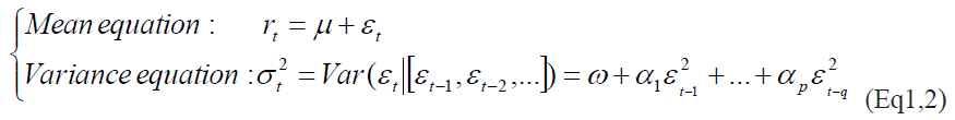
Where the residual return is defined by: is a white noise.

The conditional variance should be strictly positive at any point of time. To ensure this fact, all coefficients would be required to be non-negative: , (Brooks, 2008). In practice, a researcher usually encounters some difficulties. First, there is no clear approach that leads to determining the value of q. Second, the value of q might be very large. Third, the non-negativity constraints might be violated (Black & Scholes, 1973).

To overcome some of these difficulties, Bollerslev (1986) and Taylor (1986) had suggested generalizing the ARCH modeling. The model is known as the Generalized Auto- Regressive Conditional Heteroscedastic model (GARCH model). This model allows the conditional variance to be dependent on its own lags. The specification of GARCH model is as follows:

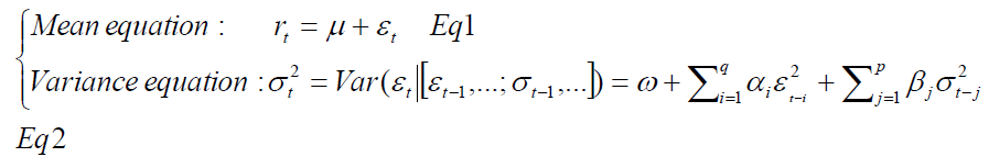
Where p is the number of lagged terms and q is the number of lagged terms. All parameters 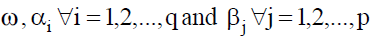should be positive to ensure the non-negativity of the conditional variance.

Although the standard GARCH model can capture several important phenomena in the financial time series, it is unable to capture other volatility properties such as leverage effects. For example, the model assumes that the effects of different shocks on volatility depend only on the size regardless of its sign. As shown in Eq. 2, the model depends on summation of square of shocks. It is well known that volatility is higher after negative shocks than after positive shocks of the same magnitude (Black, 1976), in other terms, bad news affect volatility more than good news. This has led to the use of non-linear distribution to take into account that type of stylized fact. Such non-linear models are asymmetric GARCH models, for example, EGARCH and APARCH model.

EGARCH Model

The exponential GARCH model (EGARCH) has been introduced by Nelson (1991). Contrary to GARCH model, this model can deal with leverage effects. The specification of EGARCH (p, q) is given as follows:

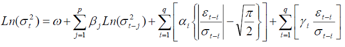
In the EGARCH model, the logarithm of the variance is modeled. Therefore, there is no need to impose the non-negativity constraints on the model parameters α, β and γ. The parameters γ measure the asymmetry or the leverage effects. The EGARCH model allows then testing the asymmetry. If then the model is symmetric and it can be reduced to symmetric GARCH model. Notice that when is positive, the total effect of 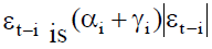whereas the total effect 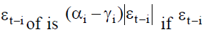is negative (Roman Kozhan, 2009). Therefore, the volatility generated by positive shocks should be less than that generated by negative shocks when In contrast, if then positive news are more destabilizing than negative news.

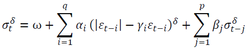
APARCH Model

The GARCH (p,q) model has been extended in various ways. Among the most interesting developments are the asymmetric power GARCH and APARCH (p,q) model (Ding, Granger & Engle, 1993), which allow taking into account both asymmetry and the possible long memory property. The APARCH model can be expressed as

The Densities

The GARCH models are estimated using a maximum likelihood (ML) approach. The logic of Maximum likelihood is to interpret the density as a function of the parameters set, conditional on a set of sample outcomes. This function is called the likelihood function.

As already noted in section 1, financial time-series often exhibit non-normality patterns, i.e. excess kurtosis and skewness. Bollerslev & Wooldridge (1988) propose a Quasi Maximum Likelihood method (hereafter QML) that is robust to departure from normality. Indeed Weiss (1986) and Bollerslev & Wooldridge (1988) show that under the normality assumption, the QML estimator is consistent if the conditional mean and the conditional variance are correctly specified. This estimator is, however, inefficient with the degree of inefficiency increasing with the degree of departure from normality (Engle & Gonz´alez-Rivera, 1991).

Since it may be expected that excess kurtosis and skewness displayed by the residuals of Conditional heteroscedasticity models will be reduced when a more appropriate distribution is used, we consider three distributions in this study: the Normal, the Student-t and the Generalizd error distribution justified by excess kurtosis (Bollerslev, 1990).

Gaussian Distribution

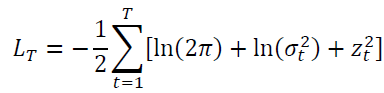
The Normal distribution is by far the most widely used distribution when estimating and forecasting GARCH models. If we express the mean equation as in equation (1) and the log-likelihood function of the standard normal distribution is given by

Student’s Distribution

Known fat tail in financial time series, it may be more appropriate to use a distribution which has fatter tail than the normal distribution. Bollerslev (1987) suggested fitting GARCH model using student t distribution for the standardized error to better capture the observed fat tails in the return series.

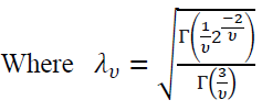
For a Student-t distribution, the log-likelihood is

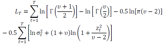
Where υ is the degrees of freedom ………, 2<υ≤∞ and Γ(.) is the gamma function. Whenυ→∞ we have the Normal distribution, so that the lower υ the fatter the tails.

Generalized Error Distribution

The log-likelihood function of the Generalized Error distribution is given by

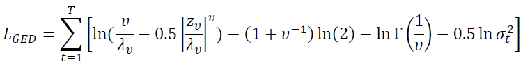
To capture the non-normal density function, the generalized error distribution was used. It’s a powerful alternative in cases where the assumption ion of conditional normality cannot be maintained. It can assume a Normal distribution, a leptokurtic distribution (fat tails) or even a palitykurtic distribution (thin tails).

Multivariate GARCH Models

This model examines the various interactions between financial time-series. It analyzes the correlations and volatility transmission from markets which are characterized by broad co-movements, especially, in periods of high financial stress, to the others markets (Silvennoinen & Teriisvirta, 2009). There are several specifications to the multivariate GARCH modelbut we will focus on the conditional correlation model.

The Dynamic Conditional correlation (DCC-GARCH) model was proposed by Engle & Sheppard (2001) and Engle (2002) to estimate large time-varying covariance matrices. This model combines dynamic correlation and the GARCH model; it is hence capable of dealing with heteroskedasticity and large dynamic covariance matrices (Engle & Bollerslev, 1986).

There are two steps in the estimation procedure. In the first step, a series of univariate GARCH models are estimated for each residual series. In the second step, standardized residuals from the first step are used to estimate parameters of dynamic correlation that are independent of the number of correlated series. This multi-stage estimation has computational advantages over multivariate GARCH models in terms of the number of parameters (Engle, 2002). The DCC-GARCH model presents a matrix of dynamic conditional correlations over time. The estimate variable is made by computing conditional volatility for a multivariate GARCH process and then using standardized residues from this model to estimate dynamic correlations. We write the model in the following form:

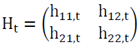
Ht=DtΓt Dt (1)

Where

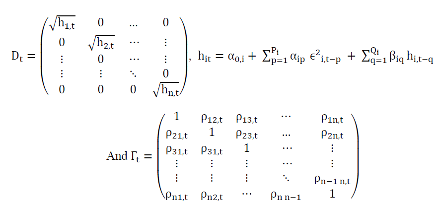
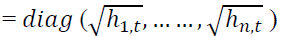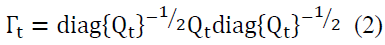
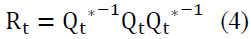
The matrix of variance-covariance must be positive and definite which implies that D_t and Γ_t should also be positive and definite since This condition is verified for D_t as it is always positive. To verify the condition on Γ_t, we have to check that 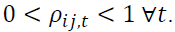To do so, we decompose the dynamic correlation matrix into the following form:

With , 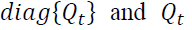are matrices that can be in rewritten under the following forms:

The condition of Q_t matrix’s definiteness and positivity imply that Γ_t is also definite and positive.

In our study, we will use the DCC-GARCH (1,1) model that we write as follows:

(3)

Where

And where

The DCC-GARCH model is a very flexible and practical model allowing the modeling of several variables with a reduced number of elements to be defined.¹

Data and Empirical Finding

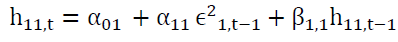
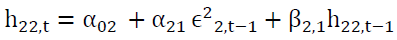
The data consist of 5757 daily observations of the S&P Sharia Index from the period December 29, 2000 to October 08, 2020 and 5760 daily observations of the Jakarta Islamic Index from the period December 29 2000 to September 30, 2020. In order to get stationary financial times series we transform prices into logarithmic returns which are presented as follows: rt= ln pt– ln where pt is the closing value of the index at date t and rt are logarithmic returns. Tables 1 and 2 present the estimation results for the parameters for GARCH, EGARCH and APARCH models with three distributions: normal, student-t and GED. Next to the parameter estimates, we report the value of the Akaike information criteria (AIC) and the value of the log likelihood (LnL).

Table 1 Parameter Estimation of Garch Models for S&P Sharia Index
	GARCH					EGARCH						APARCH
	Gaussian	Student’s	GED	Gaussian	Student’s	GED	Gaussian	Student’s	GED
ω	3.2E-06	0.000002	0.000003	-0.36493	-0.3312	-0.3511	0.00149	0.00119	0.00145
	[0.0000]	[0.0141]	[0.0079]	[0.0000]	[0.0000]	[0.0000]	[0.1886]	[0.2977]	[0.3049]
α	0.093636	0.102103	0.098654	0.094479	0.100026	0.096478	0.08091	0.089534	0.087705
	[0.0000]	[0.0000]	[0.0000]	[0.0003]	[0.0013]	[0.0047]	[0.0000]	[0.0000]	[0.0000]
β	0.887777	0.890314	0.888939	-0.17244	-0.18089	-0.18452	1	1	0.999968
	[0.0000]	[0.0000]	[0.0000]	[0.0000]	[0.0000]	[0.0000]	[0.0000]	[0.0000]	[0.0000]
γ	-	-	-	0.96647	0.970693	0.968178	0.917153	0.913448	0.913832
				[0.0000]	[0.0000]	[0.0000]	[0.0000]	[0.0000]	[0.0000]
σ	-	-	-	-	-	-	0.718628	0.754888	0.720476
							[0.0000]	[0.0001]	[0.0000]
υ	-	7.25035	1.318836	-	8.054136	1.381061	-	8.660453	1.412064
		[0.0000]	[0.0000]		[0.0000]	[0.0000]		[0.0001]	[0.0004]
LnL	3187.202	3202.858	3208.084	3214.4	3229.366	3231.887	3221.091	3233.166	3235.848
AIC	-6.04597	-6.07381	-6.08373	-6.09573	-6.12225	-6.12704	-6.10654	-6.12757	-6.13266

Table 2 Parameter Estimation of Garch Models for Jakarta Islamic Index

GARCH

EGARCH

APARCH

Gaussian

Student’s

GED

Gaussian

Student’s

GED

Gaussian

Student’s

GED

ω

0.0000011

0.0000009

0.000001

-0.234763

-0.20949

-0.223169

0.000017

0.000032

0.000025

[0.0000]

[0.0141]

[0.0006]

[0.0000]

[0.0000]

[0.0000]

[0.3069]

[0.3053]

[0.3853]

α

0.081608 [0.0000]

0.078392 [0.0000]

0.080045 [0.0000]

0.128325 [0.0003]

0.112427 [0.0000]

0.121342 [0.0000]

0.065080 [0.0000]

0.053974 [0.0000]

0.060609 [0.0000]

β

0.909979 [0.0000]

0.914805 [0.0000]

0.911975 [0.0000]

-0.071193 [0.0000]

-0.091677 [0.0000]

-0.080925 [0.0000]

0.529785 [0.0000]

0.866244 [0.0001]

0.665082 [0.0000]

γ

0.985449 [0.0000]

0.987035 [0.0000]

0.986261 [0.0000]

0.925140 [0.0000]

0.935128 [0.0000]

0.929533 [0.0000]

σ

1.470853 [0.0000]

1.308927 [0.0001]

1.375237 [0.0000]

υ

9.105655 [0.0000]

1.471618 [0.0000]

9.158047 [0.0000]

1.487143 [0.0000]

9.229091 [0.0000]

1.492968 [0.0000]

LnL

10289.2

10324.16

10326.67

10322.65

10364.99

10359.43

10325.99

10366.37

10361.3

AIC

-6.49665

-6.518102

-6.519694

-6.517151

-6.543263

-6.539754

-6.518629

-6.543507

-6.5403

The use of GARCH, EGARCH and APARCH models seems to be justified for both S&P Sharia Index and DJIM.

All α coefficients are significant at 5%. This indicates that news about volatility from the previous t periods has an explanatory power on current volatility. α Coefficients show that the current period volatility is dependent on the lagged error terms. Then, all β coefficients are significant at the 5% level. This shows that past variance terms have a strong impact on the current conditional variance and exhibit that the last period’s volatility has a significant impact on the current period conditional volatility. Moreover, the tail coefficients υ are significant which is justifying the use of non-normal densities. Finally, the leverage effect term γ in the asymmetric models EGARCH and APARCH are also statistically significant.

To compare the different models, we apply two main standard criteria: the Akaike Information Criterion (AIC) and the Log likelihood value. The AIC and the log-likelihood values reveal that the EGARCH and APARCH models estimate the series better than the traditional GARCH model. Regarding the densities, we find that Student’s and generalized error distribution clearly outperform the normal distribution. Indeed, the log-likelihood function increases when using non-normal distribution.

Consequently, APARCH (1.1) model with generalized error distribution was found to be the best model for S&P Sharia Index based on the minimum AIC and Log-likelihood value. The same model APARCH (1.1) is also found to better model the volatility of DJIM with student’s distribution instead.

Our results are showing that noticeable improvements can be made when using an asymmetric GARCH model in the conditional variance. APARCH model seems to outperform GARCH and EGARCH models. Moreover, non-normal distributions are shown to provide a better estimation than the Gaussian distribution.

We will begin our analysis by investigating the interaction between the main U.S. stock market index, the S&P 500, and its Islamic counterpart, the S&P Sharia. With Asset 1 being the conventional index and Asset 2 being its Islamic counterpart.

The results of DCC-GARCH (1.1) modeling exhibited in Table 3 show that all model coefficients are significant. Furthermore, the coefficients α₀₁ and α₀₂, which represents the minimum volatility level is very close to 0, with respectively 0.000006 for the S&P 500 and 0.000003 for its Islamic counterpart S&P Sharia. The important value of α₁₁ and α₂₁ coefficients 0.10161 for the S&P 500 and 0.10693 for its Islamic counterpart, the S&P Sharia) confirm the stock market indices' sensitivity to their shocks coinciding with the financial crisis period. We also note that both stock market indices have reached a high level of volatility persistence with a β₁₁of 0.88327 for the S&P 500 and β₂₁of 0.87516 for the S&P Sharia.

Table 3 Dcc-Garch Model Parameters for the S&P 500 and S&P Sharia
Variable	Coefficient	Std Error	T-Stat	P-value
	0.000006	0.0000007	4.28	0.000
	0.000003	0.0000007	4.40	0.000
	0.101610	0.0134200	7.57	0.000
	0.106930	0.0142200	7.52	0.000
	0.883270	0.0132100	66.85	0.000
	0.875160	0.0143700	60.88	0.000
	0.057180	0.0106000	5.39	0.000
	0.933400	0.0162100	57.55	0.000

Another observation is the high significance of conditional correlation parameters. The αDCC coefficient is close to zero with a value of 0.05718 and βDCC close to 1 with a value of 0.93340 that proves a strong conditional correlation between the two indices. These results are consistent with the empirical literature, which argues that αDCC is close to 0 and βDCC is close to 1 (Hammoudeh, Yuan, McAleer, & Thompson, 2010). The persistence of the conditional correlation calculated through the sum of αDCC and βDCC is very significant; it reaches 0.98 and close to 1. Therefore, we can argue that the two indices are strongly interdependent, especially during the financial crisis that may have played an important role as a catalyst for the volatility spillover from the conventional S&P 500 index to its Islamic counterpart, the S&P Sharia.

To expand our analysis, we will investigate this interdependence between the U.S. market represented by its main stock market index, the S&P500, and the Indonesian market represented by the Jakarta Islamic Index or JII Index.

The results of the DCC-GARCH model (1.1) presented in Table 4 exhibit significant sensitivity to past shocks and high persistence of volatility for both indices. Also, the conditional correlation parameters βDCC show a strong interdependence between the American and Indonesian markets with a high persistence reaching as high as 0.92.

Table 4 Dcc-Garch Model Parameters for the S&P 500 and JII
Variable	Coefficient	Std Error	T-Stat	P-value
	0.0000517	0.00000298	1.73	0.083
	0.0000255	0.00001400	1.83	0.068
	0.0602990	0.02790730	2.16	0.031
	0.0218602	0.07568180	2.89	0.004
	0.8846159	0.05191680	17.04	0.000
	0.6820429	0.09804490	6.96	0.000
	0.1094973	0.06764410	1.62	0.106
	0.8170304	0.09840430	8.30	0.000

To sum up, using a multivariate GARCH model (DCC-GARCH), we exhibited the existence of a strong interdependence between the U.S. stock market and Indonesian Islamic stock market. This relationship has amplified the fast contagion induced by financial globalization during the financial crisis in different Islamic markets. Despite the inherent stability characteristics of Islamic finance, we found a strong persistence of both correlation and volatility (between the U.S. stock market index and the two Islamic indexes). About these results, the stability of Islamic finance discussed widely in the literature remains relative and must be investigated further.

The widespread belief that Islamic financial markets are immune to financial shocks due to their leverage-free structure needs to be revisited. Given this conclusion, Islamic financial operators must adopt more conservative risk management practices and develop appropriate hedging mechanisms to preserve Islamic financial markets' stability in times of economic and financial uncertainty. Several mechanisms have been developed to achieve this goal, including macro-prudential policies aimed primarily at containing systemic risks and avoiding exposing the real economy to potential financial systems crises.

The modern international economy is largely an economy of interdependence, as business cycles extend across borders, and globalization pushed emerging and developing economies to adopt further economic openness. Various monetary authorities have taken several measures within the framework of macro-prudential policy to control the systemic risks resulting from this interdependence between markets. However, as shown by the COVID19 pandemic and its heavy economic fallouts, the scientific community should revisit those macro-prudential frameworks using adapted stress tests to ensure the resilience of Islamic Finance Markets.

Conclusion

In this article, we have highlighted the volatility of some Islamic stock-market indices, using heteroscedastic models. We have also highlighted the transmission of volatility from the US market to Islamic markets. The correlation between conventional and Islamic markets was very strong.

In fact, Islamic finance operates in a very complicated environment. It is exposed to interference with a large number of operators in world markets. Financial liberalization and globalization combined with the interdependence of financial markets are in particular the major challenges facing Islamic finance in order to protect itself against possible crises and against the phenomenon of financial contagion.

Faced with the problems of instability, as an exogenous factor for Islamic finance, several measures had been put in place worldwide and had given birth to the reforms developed by the Basel I, II and II committees, likely to control banking risks (the credit risk, operational risk, and market risk). These were micro-prudential reforms. However, this approach has limitations. In fact, it does not cover the systemic risks that are increasingly triggered by financial crises today. To address this problem, several approaches have been developed (macro-prudential policy in particular) with the main objective of limiting systemic risks and avoiding the exposure of the real sphere to systemic risks.

In light of this conclusion, it appears that Islamic finance operators must put in place risk management tools, design hedging mechanisms like derivatives, and preserve the stability of Islamic financial markets in period of crisis.

In fact, Risk hedging is a good way to minimize the exposure of Islamic assets to market risks. We propose in another research paper an avenue for hedging, by instrumentalising options to trade futures contracts, which mainly aim at hedging the positions of investors.

End Notes

¹Bouhali, H., Chiadmi, M.S., Ghaiti, F. (2020). Is there interdependence in foreign exchange markets during non-crisis periods? Empirical evidence from mena countries. Journal for Studies in Economics and Econometrics, 44(2), 73-108.

References

1. Baillie, R.T., & Bollerslev, T. (2002). The message in daily exchange rates: a conditional-variance tale. Journal of Business & Economic Statistics, 20(1), 60-68.
2. Baillie, R.T., Bollerslev, T., & Mikkelsen, H.O. (1996). Fractionally integrated generalized autoregressive conditional heteroskedasticity. Journal of Econometrics, 74(1), 3-30.
3. Baillie, R.T., & McMahon, P.C. (1990). The foreign exchange market: Theory and econometric evidence. Cambridge University Press.
4. Bollerslev, T., & Mikkelsen, H.O. (1996). Modeling and pricing long memory in stock market volatility. Journal of Econometrics, 73(1), 151-184.
5. Black, F. (1976). Studies of stock price volatility changes, proceedings of the 1976 meetings of the business and economic statistics section. 177-191. In American Statistical Association. sn.
6. Black, F., & Scholes, M. (1973). The pricing of options and corporate liabilities. Journal of political economy, 81(3), 637-654.
7. Bollerslev, T. (1987). A conditionally heteroskedastic time series model for speculative prices and rates of return. The Review of Economics and Statistics, 542-547.
8. Bollerslev, T. (1986). Generalized autoregressive conditional heteroskedasticity. Journal of Econometrics, 31(3), 307-327.
9. Bollerslev, T., Chou, R.Y., & Kroner, K.F. (1992). ARCH modeling in finance: A review of the theory and empirical evidence. Journal of Econometrics, 52(1-2), 5-59.
10. Bollerslev, T., Engle, R.F., & Wooldridge, J.M. (1988). A capital asset pricing model with time-varying covariances. Journal of political Economy, 96(1), 116-131.
11. Bollerslev, T. (1990). Modelling the coherence in short-run nominal exchange rates: a multivariate generalized ARCH model. The Review of Economics and Statistics, 498-505.
12. Cihak, M.M., & Hesse, H. (2008). Islamic Banks and Financial Stability: An Empirical Analysis (EPub) (No. 8-16). International Monetary Fund.
13. Coulson, N.E., & Robins, R.P. (1985). Aggregate economic activity and the variance of inflation: Another look. Economics Letters, 17(1-2), 71-75.
14. Engle, R.F. (1982). Autoregressive conditional heteroscedasticity with estimates of the variance of United Kingdom inflation. Econometrica: Journal of the Econometric Society, 987-1007.
15. Engle, R.F., Hendry, D.F., & Trumble, D. (1985). Small-sample properties of ARCH estimators and tests. Canadian Journal of Economics, 66-93.
16. Engle, R.F., Lilien, D.M., & Robins, R.P. (1987). Estimating time varying risk premia in the term structure: The ARCH-M model. Econometrica: journal of the Econometric Society, 391-407.
17. Engle, R.F., & Bollerslev, T. (1986). Modelling the persistence of conditional variances. Econometric Reviews, 5(1), 1-50.
18. Engle, R.F., & Kroner, K.F. (1995). Multivariate simultaneous generalized ARCH. Econometric Theory, 122-150.
19. Mandelbrot, B.B. (1997). The variation of certain speculative prices. In Fractals and scaling in finance. Springer, New York, 371-418.
20. Neaime, S. (2012). The global financial crisis, financial linkages and correlations in returns and volatilities in emerging MENA stock markets. Emerging Markets Review, 13(3), 268-282.
21. Nelson, D.B. (1991). Conditional heteroskedasticity in asset returns: A new approach. Econometrica: Journal of the Econometric Society, 347-370.
22. Naoui, K., Khemiri, S., & Liouane, N. (2010). Crises and financial contagion: the subprime crisis. Journal of Business Studies Quarterly, 2(1), 15.
23. Silvennoinen, A., & Teräsvirta, T. (2009). Modeling multivariate autoregressive conditional heteroskedasticity with the double smooth transition conditional correlation GARCH model. Journal of Financial Econometrics, 7(4), 373-411.