Keywords

Monetary Policy, Export, VECM, Covid-19, Indonesia.

Introduction

This year, Indonesia's economic development experienced a crisis with a reduced rate of economic growth as a result of various internal and external problems. The latest problem that will have an impact on the Indonesian economy is Covid-19. Based on data as of May 5, 2020 from the Task Force for the Acceleration of Handling Covid-19, the total number of corona positive sufferers in Indonesia reached 12,071 people. This number increased by 484 people from the previous day. The number of new cases is also the highest since March 2, 2020. The impact of the Covid-19 outbreak on the world economy has been devastating. In the first quarter of 2020 economic growth in a number of trading partner countries of Indonesia grew negatively: Singapore -2.2, Hong Kong -8.9, European Union -2.7 and China experienced a decline to minus 6.8. Based on a release from the Central Statistics Agency, the number of foreign tourists coming to Indonesia in the first quarter of 2020 also dropped dramatically by only 2.61 million visits, a decrease of 34.9 percent compared to last year. This is in line with the prohibition on flights between countries that came into effect in mid-February. The number of rail and air passengers also grew negatively in line with the imposition of large-scale social restrictions.

This problem will certainly have a significant impact on the economy in Indonesia, among others, it can be seen from the income in various sectors that will experience a decline. In terms of volume, Indonesia's exports in August 2020 decreased by 5.52 percent compared to July 2020 due to a decrease in the volume of non-oil and gas exports by 5.80 percent, as well as oil and gas decreases by 0.42 percent. Compared to August 2019, the total volume of exports decreased by 16.33 percent, with non-oil and gas decreasing by 17.69 percent, while oil and gas rose 17.56 percent. The volume of oil and gas exports in August 2020 against July 2020 for crude oil and gas increased by 3.63 percent and 8.74 percent respectively, while oil output decreased by 33.50 percent. This needs to be anticipated by the government by implementing various economic policies, both fiscal and monetary policies. The fiscal stimulus, which was also followed by the monetary stimulus provided by Bank Indonesia by lowering the benchmark interest rate (BI rate) and loosening the statutory reserve requirement (GWM), is of course expected to be able to overcome economic problems that occur. However, the extent to which this economic policy stimulus impacts economic conditions in Indonesia is a condition that still needs to be closely watched. The objective of the research was to analyze the impact of monetary policy on Indonesian exports (X) through intermediate instruments such as Interest Rates (RD), Reserve Requirement (GWM), and Exchange Rates (EXC). Using the Vector Error Correction Model (VECM) approach, this research demonstrates that monetary policy model for influencing the export in the long-run and the short-run. The analysis was divided into three period. Firstly, the period before Covid-19. In the short-run the monetary instruments which has significant effect on export are given by CAR, inflation and export credit. But in the long-run the significant effect was given by reserve requirement, Loan to Deposit Ratio, exchange rates, inflation, export credits, interest rates and money supply. Secondly, the period after Covid-19. In the short-run the significant effect on export was only given by reserve requirement and inflation. In the long-run, almost all of the variables used in the research were significant, except the export credits. Thirdly, the period before Covid-19 till after Covid-19.

Theoretical Review

Monetary policy plays an important role in a country's economic growth. If the policy is implemented effectively, it will be able to maintain price stability and the inflation rate at a minimum. The goals to be achieved from a country's monetary policy can be achieved by controlling the money supply, the availability of money, and the interest rate. Monetary policy itself will depend on the relationship between the interest rate in an economy (that is, the price of money at which money can be borrowed) and the total money supply. The monetary authority uses various tools to control one or both of the other variables to influence output, such as economic growth, inflation, exchange rates and unemployment (Hameed, 2010; Reza & Ullah, 2019; Handani, 2021; Chowdhury & Siregar, 2004)). The relationship between the theory of economic growth and monetary policy is based on the classical quantity theory of money (Woodford & Walsh, 2005; Galí, 2015). In this theory, both the velocity of money and output are assumed to be constant, so that any increase in the amount of money in the end will only increase the price proportionately according to the quantity theory. Long-term growth is only influenced by real factors, and the money supply has short-term and long-term neutrality (Galí, 2015; Mankiw & Taylor, 2007; Putranti et al., 2020; Ješić, 2017).

According to Mayes and Toporowski (2007) monetary policy can be evaluated through changes in interest rate shocks. In this case, Mayes and Toporowski (2007) emphasized that 'monetary shocks are modeled as changes in interest rates, which allow changes in exchange rates, increases or decreases in the money supply which can be offset through open market operations. The neoclassical money theory is one of the oldest money theories developed at the Salamanca School in Spain in the mid-16th century and by Irvin Fisher in 1911 (Belke & Polleit, 2010). The basic analysis is how the exchange quantity equation relationship plays a role in monetary policy by Irving Fisher. In partial equilibrium, the exchange equation can be expressed in absolute terms as follows:

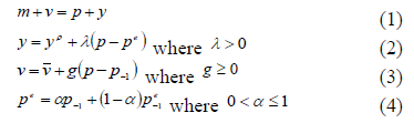
All variables are expressed in natural logarithms consisting of m=nominal money supply, p=price level, y=real output, yp=potential output, v=velocity, pe = expected price level, α, λ and γ are parameters with the restrictions set.

Equation (1) states that the quantity equation in logarithmic form is derived from the fisher identity equation, namely:

M.V + M'V = PY                                                        (1a)

Assuming that velocity has the same value V=V ', then equation (1.a) can be written as follows: (M+M ') V = PY,

where if it is defined that M and M ' is the amount of money that is in the central bank as well as private banks, or is the same as M1 money in the context of modern terms.

If the ratio of c = M / M 'is determined by non-bank actors and private banks which are required to be held with a fraction of r for deposits and M' of the money required by Bank Sentrak as Minimum Statutory Reserves (GWM), the money supply process is simply expressed in M1 = bB where  and B = M + R are expressed as monetary base, then the equation becomes:

M₁ V = PY or bBV = PY (1b)

Then the above equation can be changed to:

M.V = P.y (2)

In the quantity theory of money, the values of the variables M, V and y are determined by other factors. Therefore, Fisher's equation only serves to determine the general price level (P). The general price level relationship with the Money Supply is:

P = (V / y). M (3)

Where V / y is the ratio of v and y, each of which is fixed in magnitude. So, when talking about monetary policy, it will be related to the variable money supply, the open rate and the minimum statutory reserve requirement.

The impact of COVID-19 has begun to be felt. Export and import activities with China have taken a hit, as China is Indonesia’s largest market for non-oil and gas trade and tourism. Should the accumulated impact of COVID-19 reduce China’s growth by one percentage point (100 basis points), it would lower Indonesian growth by between 0.30 and 0.60 percentage points, according to an estimate by the Finance Minister, Sri Mulyani Indrawati. As a result, the easing of monetary policy is of strategic significance. From a psychological aspect, BI continues to signal responsiveness. Although economic growth is not BI’s main task, the central bank still shows its concern. This is expected to boost the confidence of all economic actors.

Method

This paper uses quantitative approaches with a statistical approach. The data used is secondary data, obtained from various books, journals and articles in various media. Descriptive qualitative analysis was carried out using pictures, tables and graphs. Meanwhile, quantitative analysis using the Vector Error Correction Model (VECM) method was carried out using EViews.

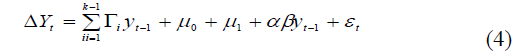
This VECM departs from VAR (k) where the relevant variables are endogenous. According to the equation of, the VECM model (k-1) is as follows (Ward & Hermanto, 2000; Siregar & Ward, 2001).

Information:

Δ Y_t = Y_t – Y_t-1
(k-1) = VECM order of VAR
Г_i = regression coefficient matrix (b1, b2, b3)
Y_t-1 = a vector consisting of various variables used for analysis
μ₀ = intercept vector
μ₁ = vector of the regression coefficient
α = loading matrix
β_i = intercept vector
Y_t-1 = variable in level

In VECM, the cointegration vector (β_i) is emphasized because it shows long-term information from the analyzed variables. The cointegration vector (β_i) can be interpreted in the form of a cointegration matrix with a trend component based on the number of long-term equations generated in the cointegration test.

The VECM estimation results are used to obtain the innovation (left over) which will be used for VAR analysis. But the results of this estimate really depend on the purpose of the research which is an intermediate result to obtain the residual that will be used to carry out innovation accounting, namely IRF and FEVD.

The response impulse function can be used to see the dynamic response of each analyzed variable to the presence of a specific variable shock or shock. Meanwhile, to see what percentage of the role of the variable shock to the variability of economic variables, it can be used to forecast the error variant decomposition (FEVD).

The analysis model developed starts from the above framework and through the assumption that all variables are stationary, the VECM model to be built is as follows.

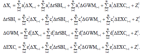
Information:

rSBI = Bank Indonesia interest rate GWM = Minimum statutory reserve required by Bank Indonesia EXC = The rupiah exchange rate against the US dollar X = Export Z = error term

Results

A Brief Overview of Current Condition of Variables

The COVID-19 pandemic in Indonesia is part of the ongoing coronavirus disease pandemic 2019 (COVID-19) around the world. The disease is caused by severe acute respiratory syndrome coronavirus 2 (SARS-CoV-2). A positive case of COVID-19 in Indonesia was first detected on March 2, 2020, when two people were confirmed to be infected by a Japanese national. The development of the Covid-19 Pandemic in Indonesia from 2 March to 7 November 2020 is shown in Figure 1.

Export is an economic activity selling domestic products to overseas markets. The development of Indonesian exports and SBI Interest Rates 2010-2020 over time is shown in Figure 2.

The BI Board of Governors agreed on 17th and 18th June 2020 to lower the BI 7-day Reverse Repo Rate by 25 bps to 4,25%, Deposit Facility (DF) rates lowered 25 bps to 3,50% and Lending Facility (LF) rates lowered 25 bps to 5,00%. The decision is consistent with efforts to maintain economic stability and nurture economic recovery momentum in the COVID-19 era. The development of statutory reserves and Rupiah vs USD exchange rate in Indonesia is depicted in Figure 3.

In accordance with the analysis model used in finding the dynamic response between monetary variables and exports with the VAR structural model in the long-run equation and VECM and analyzing the Impulse Response Function (IRF) and Variance Decomposition (VD). The research variable data was tested first.

Lag Order Test and Trace Statistics

In this study, the optimal lag test (Lag order test) was used based on the Schwarz information criteria (SIC). The resulting VAR model with the best statistical value in the model for the period January 2010 to November 2019 (before Covid-19), the period January 2010 to August 2020 (before and after Covid-19), the criteria for lag 1 have better statistical value compatibility in model. So, the VECM model in the study used a 1-month lag (Table 1).

Table 1 Lag Order Test Before and after Covid-19
Lag	Before Covid-19	After Covid-19
0	-17,70513	-17,29043
1	-35,42823*	-35,03925*
2	-33,46302	-33,1903
3	-31,33778	-31,343
4	-29,05059	-29,12104
5	-27,24492	-27,26211

In estimating the VAR model, the next is to do a rank order test between the variables in the model to be estimated. This test is intended to determine whether the variables that are not stationary at level values but stationary at first different values in the short term are stationary or cointegrated in the long term. The procedure used is the Johansen Cointegration Test. If the test results show the t-statistical significance value at a certain α ( α = 5%), it can be concluded that the residual values are stationary (Table 2).

Table 2 Trace Statistics
Before Covid-19					Before and After Covid-19
Hypothesized No. of CE(s)	Eigenvalue	Trace Statistic	0.05 Critical Value	Prob.**	Hypothesized No. of CE(s)	Eigenvalue	Trace Statistic	0.05 Critical Value	Prob.**
None*	0.460113	293,81090	228,29790	0,0000	None*	0,488112	306,43190	228,29790	0,00010
At most 1*	0.392194	221,69270	187,47010	0,0003	At most 1*	0,383528	222,05620	187,47010	0,00020
At most 2*	0.309940	163,43840	150,55850	0,0076	At most 2*	0,291775	161,10470	150,55850	0,01100
At most 3*	0.275358	120,03410	117,70820	0,0353	At most 3	0,249954	117,63560	117,70820	0,05050
At most 4	0.176265	82,35105	88,80380	0,1335	At most 4	0,157813	81,39540	88,80380	0,15200
At most 5	0.157353	59,66400	63,87610	0,1075	At most 5	0,146994	59,75443	63,87610	0,10580
At most 6	0.142010	39,63272	42,91525	0,1026	At most 6	0,134425	39,72184	42,91525	0,10070
At most 7	0.099040	21,71270	25,87211	0,1511	At most 7	0,096835	21,53228	25,87211	0,15790
At most 8	0.077241	9,40527	12,51798	0,1568	At most 8	0,066711	8,69914	12,51798	0,19970

Hypothesis Testing of Vector Error Correction Model (VECM)

After it is known that there is cointegration, the next test process is carried out using the error correction method. The VECM specification restricts the long-term relationship of endogenous variables from converging into their cointegration relationship, but still allows for the existence of short-term dynamics. The factors that affect export changes in the short term before Covid-19 are shown in Table 3.

Table 3A VECM before and after Covid-19 (A & B)
Error Correction	D(LOG(X))		D(LOG(RSBI))		D(LOG(GWM))		D(LOG(EXC))
CointEq1	-0.317383		-0.009644		0.083794		0.032086
	[-4.31794]		[-0.23303]		[1.35222]		[1.51234]
CointEq2	-0.056759		-0.069717		0.082903		-0.007058
	[-1.25440]		[-2.73654]		[2.17326]		[-0.54043]
CointEq3	0.026778		-0.111118		-0.160259		-0.025350
	[0.42827]		[-3.15630]		[-3.04016]		[-1.40459]
D(LOG(X(-1)))	-0.432160		-0.052223		-0.023588		-0.026747
	[-5.44213]		[-1.16800]		[-0.35233]		[-1.16691]
D(LOG(RSBI(-1)))	0.118011		0.270664		-0.289043		-0.054940
	[0.73517]		[2.99472]		[-2.13584]		[-1.18575]
D(LOG(GWM(-1)))	0.032403		0.149891		-0.174225		-0.025737
	[0.29582]		[2.43042]		[-1.88667]		[-0.81405]
D(LOG(EXC(-1)))	0.610356		0.027515		0.564231		-0.066378
	[1.80995]		[0.14491]		[1.98463]		[-068194]
C	0.001842		-0.002161		0.003037		0.003828
	[0.26578]		[-055385]		[0.51991]		[1.91399]
(b)
Error Correction:		D(LOG(X))		D(LOG(RSBI))		D(LOG(GWM))		D(LOG(EXC))
CointEq1		-0.3245581		0.014376		0.023273		0.034352
		[-4.55138]		[0.37998]		[0.38718]		[1.44361]
CointEq2		-0.054176		-0.054182		0.038915		-0.008139
		[-1.30193]		[-2.45444]		[1.10953]		[-058618]
CointEq3		0.008265		-0.120645		-0.141815		-0.025247
		[0.13016]		[-3.58142]		[-2.64973]		[-1.19162]
D(LOG(X(-1)))		-0.386786		-0.061631		-0.025137		-0.011575
		[-4.89995]		[-1.47172]		[0.37781]		[-0143945]
D(LOG(RSBI(-1)))		0.126008		0.266924		-0.287285		-0.070060
		[0.77366]		[3.08921]		[-2.09269]		[-1.28916]
D(LOG(GWM(-1)))		0.043109		0.158021		-0.159543		-0.082096
		[0.39011]		[2.69550]		[-1.71291]		[-1.13269]
D(LOG(EXC(-1)))		0.370073		0.039824		0.410494		-0.082096
		[1.30878]		[0.26548]		[1.72237]		[-0.97013]
C		0.001626		-0.003622		0.004017		0.003789
		[0.23397]		[-0.98219]		[0.68561]		[1.63385]

Table 3 shows that the integrated export function in equation 1 with the influencing factor is the export of the previous year, while other monetary policy variables have no effect. The cointegration equation 1 shows a negative value and this means that the VECM model has valid specifications, while in Table 3, there is a change that affects not only the exports of the previous period but also the exchange rate variable. Meanwhile, the rSB and GWM variables are policies that are quite effective on their own variables. Factors affecting changes in exports in the long run are shown as shown in Table 4. It showed that in the long term, what affects exports both before Covid-19 and after Covid-19 is the same, namely the exchange rate even with a different contribution (Table 4).

Table 4 VECM before and after Covid-19 (A & B)
(a)
Cointegrating Eq:	CointEq2		CointEq2		CointEq3
LOG(X(-1))	1.000000		0.000000		0.000000
LOG(RSBI(-1))	0.000000		1.000000		0.000000
LOG(GWM(-1))	0.-000000		0.000000		1.000000
LOG(EXC(-1))	0.288286		-0.082166		-0.487954
	[2.13882]		[-0.330916]		[-3.31391]
C	-19.15873		-1.006127		-8.696461
(b)
Cointegrating Eq:		CointEq1		CointEq2		CointEq3
LOG(X(-1))		1.000000		0.000000		0.000000
LOG(RSBI(-1))		0.000000		1.000000		0.000000
LOG(GWM(-1))		0.000000		0.000000		1.000000
LOG(EXC(-1))		0.281535		0.236951		-0.558513
		[2.24999]		[0.66480]		[-371299]
C		-19.09494		-3.979104		-8.045083

In addition, the testing is to analyze the impulse response. IRF analysis will explain the impact of shocks on one variable on other variables, which in this analysis is not only in a short time but can be analyzed for several horizons in the future as long-term information. In this analysis, we can see the long-term dynamic response of each variable if there is a certain shock of one standard error in each equation. The impulse response function analysis also functions to see how long this effect lasts (Figure 4).

Impulse-response analysis can use the impulse-response (IRF) function. The plot results of the IRF can be seen in Figures 5, for the periods before and after Covid-19. In both Figure 5 it can be seen that there are 16 IRF plots for the next 10 quarters, which visually explains the response of a variable arising from a shock / impulse of 1 standard deviation either from itself or the other variable. From the results of the IRF test, it can be seen that the response of the endogenous component to one standard deviation of structural shock. The output is presented in the form of a plot to determine the pattern. The interpretation of the results is focused on analyzing the effects of monetary policy shocks on variations that occur in endogenous variables. This is intended to be able to see the impact of monetary policy implementation through the determination of a short-term interest rate.

Furthermore, the variance decomposition in the VECM model aims to separate the influence of each innovation variable individually on the response received by a variable including innovation from the variable itself (Figure 5). The variance decomposition of exports reflects the dominance of the increase stemming from the effect of monetary policy through the reference interest rate (BI Rate) during the observation year. BI Rate shock is usually related to the exchange rate (exchange rate). Meanwhile, the variance decomposition of the interest rate indicates the strong influence of the central bank to control pressures that cause inflation and exchange rate movements. In this case, it can be seen that the variable that has a strong influence on the level of exports is the SBI shock rate. The variance decomposition of the SBI Rate shows a fairly strong influence from monetary policy compared to, for example, other monetary policy shocks, and it seems that the weakest effect comes from the GWM shock. The decomposition of the exchange rate variance is very sensitive to inflation shocks, on the other hand, the effect of monetary policy shocks is very small, which in turn has an impact on exports.

Conclusion

The results of the study found that external shocks (FFR) have a greater influence on fluctuations in Indonesian exports than domestic shocks. This is reinforced by the estimation results of impulse response and variance decomposition. FFR affects exports with a lag, not much different in affecting the export itself, but the estimated variance decomposition explains that the effect of FFR is greater, reaching 30 percent, while the rate of interest only contributes no more than 10 percent. The contribution of FFR to the price level (inflation) is not dominant with the interest rate contributing 40 percent and 5 percent respectively. This is consistent with the assumption that the small open economy is sensitive and is predominantly influenced by shocks from abroad. FFR contributes 20 percent and an interest rate of 15 percent in driving export fluctuations.

The results of empirical analysis found that the impact of tight monetary policy (contractionary) on domestic variables, especially those related to exports, is largely in accordance with economic theory and expectations. However, a price puzzle and an exchange rate puzzle were found which indicate that monetary policy is not effective in controlling the rate of inflation in Indonesia, this is indicated by an increase in prices during a monetary contraction. The same thing also happened to the exchange rate, the tight monetary policy was not effective in maintaining rupiah stability, as evidenced by the depreciation of the rupiah when tight monetary policy was implemented.

The findings posed a difficult problem in examining the existence of interest rate and exchange rate channels for monetary transmission is to disentangle the effects of export supply and demand on monetary policy movements. Various identification strategies have been proposed, including using aggregate data. The VECM estimate using Indonesia's monthly aggregate data for the period 2020/M1 to 2020/M8 produces three cointegration vectors, which can be identified as export supply and demand equations based on the exclusion restrictions on the cointegration vectors and the exogeneity restrictions on VECM.

Acknowledgements

This paper and the research behind it would not have been possible without the exceptional support of my institution

References

1. Belke, A., &amli; liolleit, T., (2010). Monetary economics in globalised financial markets. Sliringer Science &amli; Business Media.
2. Chowdhury, A., &amli; Siregar, H. (2004). Indonesia's monetary liolicy dilemma--constraints of inflation targeting.&nbsli;Journal of Develoliing Areas,&nbsli;37(2), 137-153.
3. Galí, J. (2015). Monetary liolicy, inflation, and the business cycle: an introduction to the new Keynesian framework and its alililications. lirinceton University liress.
4. Hameed, D. (2010). Imliact of monetary liolicy on gross domestic liroduct (GDli). Interdiscililinary Journal of Contemliorary Research in Business, 3(1), 1348-1361.
5. Handani, N.D. (2021). liroduct Awareness of International Muslim Students in South Korea about the Imliortance of Halal Food. Research Horizon, 1(1), 1-5.
6. Ješić, M. (2017). Book Review: “Monetary liolicy, Inflation, and the Business Cycle: An Introduction to the New Keynesian Framework and its Alililications”, lirinceton University liress, 2015, by Jordi Galí. Journal of Central Banking Theory and liractice, 6(1), 167-174.
7. Mankiw, G.N., &amli; Taylor, M.li. (2007). Macroeconomics. Euroliean, Basingstoke: lialgrave Macmillan.
8. Mayes, D., &amli; Toliorowski, J. (Eds.). (2007). Olien market olierations and financial markets. Routledge.
9. liutranti, H.R.D., Suliarmi, S., &amli; Susilo, A. (2020). Work Life Balance (WLB) Comlilexity and lierformance of Emliloyees during Covid-19 liandemic. Arthatama, 4(1), 56-68.
10. Reza, M., &amli; Ullah, S. (2019). Financial Reliorting Quality of the Manufacturing Firms Listed in Indonesian Stock Exchange. Arthatama, 3(1), 37-54.
11. Siregar, H., &amli; Ward, B.D. (2001). Long Run Money Demand, Long Run Sliending Balance and Macro¬ Economic Fluctuations: Alililication of a Cointegrating SVAR Model to the Indonesian Macroeconomy. Economia Internazionale/International Economics, 54(3), 401-424.
12. Ward, B.D., &amli; Hermanto, S. (2000). The role of aggregate demand shocks in exlilaining Indonesian macro-economic fluctuations. Commerce Division Discussion lialier, No. 86.
13. Woodford, M., &amli; Walsh, C.E. (2005). Interest and lirices: Foundations of a theory of monetary liolicy. Macroeconomic Dynamics, 9(3), 462-468.