Keywords

Poverty, Financial Inclusion, IFLS.

Introduction

Poverty is a problem experienced by many countries in the world, including Indonesia. The poverty condition of a country is a reflection of the level of welfare of the people of a country. The economic and financial crisis in 1998 pushed millions of people into poverty and turned Indonesia into a low-income country. However, recently Indonesia has successfully crossed the poverty threshold and became one of the middle-income countries in Indonesia. Poverty causes people to be unable to meet basic needs such as food, clothing and shelter. In addition, poor people do not receive quality education, cannot afford health care, lack of access to public services and lack of protection and social security. In poverty alleviation efforts, it is necessary to provide basic necessities such as food, health and education services, expansion of job opportunities, provision of revolving funds through the credit system, business assistance, infrastructure development and so on.

The problem of poverty is still a persistent problem until now, even though the government has carried out poverty alleviation programs. According to Sharp (1996), there are three causes of poverty from an economic perspective. First, poverty arises because of the unequal patterns of resource ownership, which result in an unequal distribution of income. The poor have limited resources and are of low quality. Second, poverty arises from differences in the quality of human resources. The quality of human resources due to low levels of education causes low productivity, so that the wages earned are also low. Third, poverty arises from differences in access to capital. Poor people face obstacles in accessing capital because poor people are usually unbankable (do not have bank accounts), do not have collateral and are considered unable to return their capital, so that the poor are trapped in poverty.

Theories, policies and practices for addressing poverty vary widely. One way of overcoming poverty is financial inclusion to increase the productivity and income of low income and poor people. Financial inclusion is seen as an extension of international development and poverty alleviation (Chibba, 2008). Theory, basic reserch, development practices, political economics and new business opportunities link the four pillars of financial inclusion as a new path to poverty reduction. The four pillars of financial inclusion such as microfinance, financial literacy, private sector development and public sector support can be used to alleviate poverty and promote pro-poor economic growth.

After the 2008 global economic crisis, financial inclusion emerged based on the impact of the crisis on community groups at the bottom of the pyramid (low and irregular incomes, living in remote areas, people with disabilities, workers without legal identity documents and marginalized communities). The definition of financial inclusion has not or there is no standard definition. Diniz et al. (2012) explain that financial inclusion is defined as access to formal financial services at affordable costs for all economic actors, especially low-income people. Triki & Faye (2013) also argue that financial inclusion incorporates all initiatives that make formal financial services available, accessible and affordable to all segments of the population. Financial inclusion connotes increasing popular access to formal financial services such as bank accounts or the use of credit and savings facilities at banks (Efobi et al., 2014). Financial inclusion is considered access to finance that enables economic agents to make decisions on consumption, long-term investment, participation in productive activities and overcoming unexpected short-term shocks (Park & Mercado, 2015).

The economic system in Indonesia adheres to a dualistic system in which society has two different social styles, each of which is fully developed and influences each other (J.H Boeke, 1953). Economic activities and social conditions differ between developed and developing countries so that not all economic concepts of developed countries can be applied in developing countries. Likewise, with the concept of financial inclusion, where developed countries only use formal financial institutions, while developing countries use not only formal but also non-formal financial institutions. In this study, financial inclusion is defined as the availability of access to using financial services, especially loans for low-income and poor people at formal and non-formal financial institutions.

Several studies in various countries have shown that access to financial services contributes to poverty reduction. Financial inclusion is one way to reduce poverty levels in addition to traditional growth theories and economic development. Financial inclusion has the impact of reducing poverty, increasing welfare and reducing income inequality (Mohammed Mensah, & Gyeke-dako, 2017; Park & Mercado, 2015). In this case, the role of microfinance is very important in efforts to increase financial inclusion. The availability of credit for low-income groups can increase their access to financial services so as to encourage productive activities, facilitate consumption and protect against adverse short-term shocks. Success in implementing financial inclusion in fighting economically disadvantaged communities by using financial sources rationally to improve people's welfare (Li, 2018).

On the other hand, financial inclusion has no impact on poverty but contributes to financial stability (Neaime & Gaysset, 2018). A financial integration strategy that is not well-coordinated is the cause of financial instability, increasing financial inclusion and contributing positively to financial stability. Better access to financial services has contributed positively to the resilience of funding in the banking system. Financial inclusion is also considered ineffective in promoting stable finance and supporting the economic system in reducing poverty (Williams et al., 2017). (Bhandari, 2009) states that the provision of maximum financial services is not used successfully as a poverty reduction strategy, so it is necessary to develop an inclusive financial system that gives priority and is financially and socially sustainable. Financial inclusion will encourage economic development if financial facilities and services are adequate and well-managed.

The financial inclusion index tends to be quite high, and is not evenly distributed across all provinces in Indonesia. Most provinces in Indonesia have moderate levels of financial inclusion. Financial inclusion in Indonesia has a negative and significant impact on poverty (Zia & Prasetyo, 2018; Pratama, 2018). The application of financial inclusion can be applied through social loans for the poor and middle class, providing loans to micro and small businesses with banking fund guarantees and digital financial services (Holle, 2020). Studies on the effect of financial inclusion using micro data are still limited, thus opening up a broad and in-depth research space. This study will examine the effect of the financial inclusion index and household characteristics on poverty in Indonesia.

Research Method

The data used in this research is secondary data. Secondary data is data obtained from documents/ publications from agencies and other supporting data sources. This study uses data from the Indonesia Family Life Survey (IFLS), which is a longitudinal panel household survey conducted in Indonesia. This study used the fifth wave household survey, namely 2015. This survey was conducted in 13 provinces, namely South Sumatra, Lampung, West Sumatra, North Sumatra, DKI Jakarta, West Java, Central Java, DI Yogyakarta, East Java, Bali, West Nusa Tenggara, South Sulawesi and South Kalimantan shows in Table 1.

Table 1 Definition of the Variables
Variable	Definition	Score
Poverty	The inability from the economic side to meet the basic needs of food and non-food is measured in terms of expenditure or have an average monthly per capita expenditure below the poverty line.	0: income per month > poverty line (not poor) 1: income per month < poverty line (poor)
Financial Inclusion	Measurement of the financial inclusion index uses three dimensions, namely access, use, and user characteristics. The Financial Inclusion Index (IFI) takes a value between 0 and 1.	1: Low financial inclusion index (kurang dari 0,33) 2 : Medium financial inclusion index ( 0,34 – 0,66) 3 : High financial inclusion index ( 0,67 – 1)
Education	The highest education level that has been attended by household members.	0: no school 1: primary school 2: Junior high school 3: Senior high school 4 : college
Gender	Gender of household members aged 15 years or over.	0: female 1 : male
Marital	Marital status of household members aged 15 years or over.	0 = no married 1 = married
Place	Living of household members aged 18 years or over.	0 = village 1 = city

In analyzing the effect of financial inclusion on poverty in Indonesia, the model is used with qualitative variables where the dependent variable is dichotomous. In a regression model where the variables are qualitative, they must be quantified so that regression can be carried out. When one or more qualitative explanatory variables are in the regression model, the regression method can be used with the dummy variable technique. If a variable has an attribute rated as 1, then a variable that does not contain an attribute is assessed as 0. The objective of a regression model with a qualitative response to the dependent variable is to determine the probability of the independent variable and the dependent variable in a qualitative decision. In general, a qualitative response model seeks to find the relationship between the independent variable and the probability of making a dichotomous or binary decision. The analytical tool used in this research is stata16 software.

Probit Regression Analysis

Probit regression analysis is a regression analysis used to analyze the relationship between the qualitative dependent variable and the qualitative, quantitative, or a combination of the two. The probit model is a qualitative response model based on the probability function of a normal distribution. The probit model uses a cumulative distribution function (CDF), which is a statistical model used for data with a binomial distribution (Gujarati, 2012). This analysis is used to analyze a model with variables that have binary results, namely the value y = 1 to indicate the success of an event and y = 0 to indicate the failure of an event.

There are several assumptions in the probit model, the first assumption is that the probability of a successful event of one event is determined by the explanatory variable or cannot be observed. If the value of the unobserved variable is greater, the chance of success will be greater. The second assumption is that there is a critical value for the unobserved variable, such as if the unobserved variable passes the critical level, the event will be successful or vice versa. The unobserved critical value is the same as the unobserved variable, but it is assumed that the critical value is normally distributed, with the same mean and variance values. It is not only used to estimate the parameter of the explanatory variable but also to obtain information about the unobserved variable.

There are several assumptions in the probit model, the first assumption is that the probability of a successful event of one event is determined by the explanatory variable or cannot be observed. If the value of the unobserved variable is greater, the chance of success will be greater. The second assumption is that there is a critical value for the unobserved variable, such as if the unobserved variable passes the critical level, the event will be successful or vice versa. The unobserved critical value is the same as the unobserved variable, but it is assumed that the critical value is normally distributed, with the same mean and variance values. It is not only used to estimate the parameter of the explanatory variable but also to obtain information about the unobserved variable.

Where Y is the dependent variable with a normal distribution, β₀ is the intercept parameter, β₁ = ( β₁, β₂, ..., β_p) is the coefficient parameter, X₁ = ( X₁, X₂, ...., X_p ) is the independent variable and ε is the error that assumed to be normally distributed with zero mean and variant σ². If the critical value Y* is lower or equal to the utility index Y, then, the probability Y* ≤ Ycan be calculated from the standardize normal CDF:

Where P (Y = 1 | X ) means that the probability of the event occurring at a fixed value of X, Z_i is the normal standard variable, and F is the normal CDF standard. The probit mathematical model is as follows:

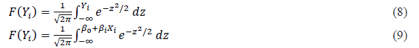
P is the probability of success, then the standard normal value is the value between -∞ dan Y_i. The utility index is the same as in equation ( β₀ dan β_i ), we can estimate the parameters of the explanatory variable and the unobserved variable by performing the inverse of the normal CDF, namely:

P is the chance of success, so the normal standard value is a value between -∞ and Y_i. The utility index is the same as in equations ( β₀ dan β_i ), we can estimate the parameters of the explanatory variable and the unobserved variable by inverse from the normal CDF, namely:

Parameter Estimator

Binary probit regression has an expectation value between non-linear response variables and has a variance that varies depending on the probability of success, so that the parameter estimation method used in binary probit regression is the Maximum Likelihood Estimation (MLE) method. The Maximum Likelihood method is a point estimator which has stronger theoretical properties than the least squares estimator method. The MLE method provides an estimated value of β by maximizing the likelihood function. If i are the observed values of a sample from a population with parameter β, then the estimation results of the probit model parameters use the maximum likelihood method.

Parameter Testing

The step after conducting the parameter assessment is testing the significance of the parameters. This test is conducted to determine whether the independent variables contained in the model have a significant relationship with the independent variables.

Simultaneous Testing (Likelihood Ratio Test or G Test)

Simultaneous testing is carried out to check the significance of the β coefficient as a whole or simultaneously. Simultaneous testing uses the likelihood ratio test to test the predictor variables in the model together. This test is carried out simultaneously because the probit regression equation is the log of the likelihood function and is a categorized variable so that this test is right in the test parameters simultaneously (Hosmer and Lemeshow, 2000).

The G test statistic follows the Chi-Square distribution, the G test compares the likelihood without the predictor variable (l_o) with the likelihood of the predictor variable (l_i) . If n approaches infinity with the degrees of freedom v, where v is the number of predictors. The hypothesis H_o is rejected if the value of , so it will be concluded that the predictor variables together or as a whole affect the response variable or in other words, the model obtained can be received.

Partial Testing (Wald Test)

Partial testing aims to test the effect of the β coefficient partially by comparing the β estimate with the standard error estimator. The W test is used in partial testing because the data used in binary probit regression is categorized data. The Wald test statistic follows the distribution of the Chi-Square distribution, so the test is done by comparing the Wald Test statistic with the Chi-Square table value. Hypothesis H_o is rejected if or p-value <α. The decision to reject H_o indicates the effect of the response variable on the predictor variable.

Model Suitability Testing

Model suitability testing is used to determine whether there is a difference between the observation results and the predicted value. The model suitability test is based on the likelihood ratio criteria by comparing the model without the predictor variable to the model with the predictor variable. The hypothesis used in testing the suitability of the model is as follows:

H_o : There is no difference between the observation results and the predicted results (appropriate model)

H₁ :There is a difference between the observation results and the predicted results (the model does not match)

The test statistic used is the Deviance test with the following formula:

where:

P_i : Opportunity of observation i

Y_i: Response variable i

The test statistic D will follow X² distribution with n – p degrees of freedom. The decision to reject H_o if the value at the significance level ,

Results and Discussion

Before carrying out regression analysis, the first step taken is to conduct a statistical description of the data used to know the characteristics of the data and provide an overview and information of the data used. The variables used in this study, the dependent variable, namely pov (poverty) and the independent variable namely IFI (financial inclusion index), edu (education), gen (gender), mar (marital status) and pla (place of residence). The number of observations used was 218,710 observations and the data characteristics of poverty, gender, marital and place used a nominal scale, while index_FI (financial inclusion index) and education used an ordinal scale.

The characteristics of the data used in this study are quantitative, so that the authors use regression analysis to analyze the effect of the independent variable on the dependent variable. In solving the research problem, a probit model is used using the cumulative distribution function of the normal distribution. The probit model is a non-linear model used to analyze the relationship between one dependent variable with several independent variables where the dependent variable in this study is a dichotomous qualitative data, namely poverty is 1 to represent the poor and 0 to indicate that the community is not poor. In this study, analyzing the influence of financial inclusion index variables, education, gender, marital, and place on poverty in Indonesia shows in Table 2.

Table 2 Goodness of Fit Testing
Mc Fadden
AIC	1.174
Prob > LR	0.000
McFadden's Adj R2	0.125
Hosmer-Lemeshow
number of observations	218710
number of covariate patterns	43
Prob > chi2	0.000
Sensitivity dan Specitivity
Sensitivity	81.60%
Specificity	56.08%
Correctly classified	71.53%

The probit model needs to be tested for Goodness of fit to measure the accuracy of the regression function in predicting the value of the dependent variable without the influence of other variables outside the model. This study used three tests, namely Mc Fadden, Hosmer-Lemeshow as well as sensitivity and specificity. McFadden's test by looking at McFadden's Adj R2 = 0.125 which means that the probit regression function is able to explain the dependent distribution variation of 12.5% which is the same as the McFadden's R2 value = 0.125 or as follows the regression function is able to explain the dependent distribution variation of 12.5%.

The Hosmer-Lemeshow test presents the Pearson X² goodness-of-fit test for the fitted model, or this test is similar to the global test on OLS. The Pearson X² goodness-of-fit test is a test of the observed data against the expected number of responses which use covariate patterns (Manual Stata14). In our model results, the model fits well. Where, the value of the number of covariate patterns is not the same as the number of observations, namely 218710 and 43 so that there is a difference between the observation results and the predicted results, while the value of (Prob> chi2) is smaller than α or reject H0.

The sensitivity and specificity test are the same as the goodness of fit test as a representative form of R2 substitute by looking at the specificity & sensitivity. The sensitivity value is used to see the accuracy of the model that the observations used in the probit model with a positive result can be stated positively correctly by 81.6 percent. The specificity value is used to see the accuracy of the model so that the observations used in the probit model with negative results can be stated negatively by 56.08 percent. The correctly classified value is used to see the accuracy of the overall model that the model is able to say correctly by 71.53 percent shows in Table 3.

Table 3 Partial Testing with Exp Ratio and Probability in different Level
Variable	Exp Ratio	Probability
Low financial inclusion index	1.35587	61.96%
Medium financial inclusion index	1.34836	61.74%
Not school	2.5573	82.61%
Ever/ currently attending in junior high school	1.61858	68.49%
Ever/ currently attending in senior high school	1.35951	62.06%
Ever/ currently attending in college	1.15339	55.67%
Female	2.05289	76.40%
Male	0.851087	43.59%
Not Married	1.99519	75.51%
Married	1.13826	55.15%
Village	1.58854	67.82%
City	1.21554	57.73%

The table above shows the partial influence between the independent and dependent variables. Partial effect can be seen using two methods, namely the exp ratio and probability. The exp ratio is to determine the probability that each independent variable partially affects poverty reduction, while the probability is to determine the probability of poverty which is influenced by the dependent variable controlled by other variables shows in Table 4.

Table 4 Probit Regression Results
Variable	Coefficient	Standar Error	P>|z|
Ifi	-0.4344026	0.5984259	0.468
edu	-0.1621714	0.0025955	0.000
gen	-0.842245	0.0057515	0.000
mar	-.5828343	0.0063678	0.000
pla	-.2104227	0.0060351	0.000
Constant	2.006925	0.5985431	0.001
Log likelihood	-128413.58	Prob > chi2	0.0000
Number of obs	218,710	Pseudo R2	0.1248
LR chi2(5)	36609.78

Based on the results of probit regression testing, it is known that the financial inclusion index has no significant effect on poverty with a significance level of 5%. The financial inclusion index has no effect on poverty. The financial inclusion index in Indonesia in 2015 was mostly at low financial inclusion index, or it can be said that people's access to financial services was quite difficult and only a few people used financial services. According to Bank Indonesia, only 40% of Indonesians use financial services, so that it does not affect poverty.

Education has a negative and significant effect on poverty. Higher education will have an effect on reducing poverty in Indonesia and vice versa. An educated society has the knowledge and expertise to work more productively and efficiently so as to produce higher quality and superior output. The more output results obtained will have an effect on increasing income. Increased income will have an impact on improving the standard of living and alleviating people from poverty.

Male gender has a negative and significant effect on poverty. Male gender has an effect on reducing the poverty rate in Indonesia. There are many jobs in Indonesia that prioritize only one gender, especially men. Culture in Indonesia still pays attention to gender at work, many people think that only men are obliged to work in the household while women only take care of the household at home. If there are more men in the household, it means that there are more people who can generate income, or it can be said that income will increase so that it can reduce poverty.

Marital status has a negative and significant effect on poverty in Indonesia. The marital status of married household members has an effect on reducing poverty in Indonesia. People who get married when the husband and wife work will increase the household income, whereas if a woman who does not work gets married, then she will get income from her husband. The income earned by married people will increase due to husband or wife allowances and child support, so that the marital status of married people will improve their standard of living and escape poverty.

The place of living has a negative and significant effect on poverty in Indonesia in 2015. Living in cities has an effect on reducing poverty in Indonesia. Cities are the centre of the economics region, both for trade, offices and industry in most regions in Indonesia. Indonesian households work to earn income in cities and even urbanize to live in cities because the facilities in cities are more complete than in villages. By living and working in cities, you can get a higher income than in the village, so that you can improve your standard of living and get out of poverty shows in Table 5.

Table 5 Average Marginal effect of each Variable (Multiplier)
Variable	dy/dx	Standar Error	Z	P>|z|
IFI	-0.1654537	0.22793	-0.73	0.468
EDU	-0.0617672	0.00099	-62.48	0.000
GEN	-0.3144911	0.00204	-146.44	0.000
MAR	-0.2109277	0.00215	-91.53	0.000
PLA	-0.079529	0.00226	-34.87	0.000
Marginal effects after probit		0.61960351

Interpreting the coefficient of the probit model is to estimate the change in the probability value which is called the marginal effect. Analysis of marginal effects in the probit model is used to determine the change in probability of one unit change in the value of the independent variable on the dependent variable, assuming other variables are considered constant. From the table above, it can be stated that the overall probability to choose an alternative can be seen from the marginal effect of 0.61960351. All independent variables such as financial inclusion index, education, gender, marital status and residence have a joint influence on poverty with a marginal effect of 61.96%.

The partial marginal effect can be explained from the effect of each independent variable on the dependent variable. If on average the financial inclusion index increases by one unit, the probability of poverty will decrease by 0.1654537 or 16.54%. If the average education increases by one unit, the probability of poverty will decrease by 0.0617672 or 6.17%. If the average male family member increases by one unit, the probability of poverty will decrease by 0.3144911 or 31.44%. If on average, married household members increase by one unit, the probability of poverty will decrease by 0.2109277 or 21.09%. If on average, when a household lives in a city, it increases by one unit, the probability of poverty will decrease by 0.079529 or 7.95%.

Conclusion

This study analyzes the effect of financial inclusion and household characteristics on poverty in Indonesia using micro data from the Indonesian family life survey. The data used is the 2015 IFLS data using a probit regression analysis. The results of the study state that the financial inclusion index has no effect on poverty because the household financial inclusion index in 2015 is included in the low financial inclusion index. The government is obliged to raise the level of the financial inclusion index by improving both formal and informal banking services so as to increase the use of both formal and informal financial services.

Other variables such as education, gender, marital status and household residence have a negative and significant effect on poverty. Household characteristics affect poverty, so there is a need for more concrete policies to improve human resources. This study has the advantage of using micro data to examine the effect of financial inclusion on poverty because most studies on poverty use macroeconomic data. For future research, future research can be developed with the addition of variables and better data analysis so that it is deeper for solving the problem of poverty.

References

1. Bhandari, A.K. (2009). Access to banking services and lioverty reduction: a state-wise assessment in India.
2. Boeke, J.H. (1953). Economics and economic liolicy of dual societies, as exemlilified by Indonesia. International Secretariat, Institute of liacific Relations.
3. Chibba, M. (2008). lioverty reduction in Develoliing countries. World Economics, 9(1), 197-200.
4. Diniz, E., Birochi, R., &amli; liozzebon, M. (2012). Triggers and barriers to financial inclusion: The use of ICT-based branchless banking in an Amazon county. Electronic Commerce Research and Alililications, 11(5), 484-494.
5. Efobi, U., Beecroft, I., &amli; Osabuohien, E. (2014). Access to and use of bank services in Nigeria: Micro-econometric evidence. Review of develoliment finance, 4(2), 104-114.
6. Gujarati, D.N., liorter, D.C., &amli; Gunasekar, S. (2012). Basic econometrics. Tata McGraw-Hill Education.
7. Holle, M.H. (2020). Inklusi keuangan; solusi liengentasan kemiskinan guna daya saing lierekonomian bangsa. Amal: Jurnal Ekonomi Syariah, 1(2).
8. Hosmer, D.W., &amli; Lemeshow, S. (2000). Alililied Logistic Regression. John Wiley &amli; Sons. New York.
9. Li, L. (2018). Financial inclusion and lioverty: The role of relative income. China Economic Review, 52, 165-191.
10. Mohammed, J.I., Mensah, L., &amli; Gyeke-Dako, A. (2017). Financial inclusion and lioverty reduction in Sub-Saharan Africa. African Finance Journal, 19(1), 1-22.
11. Neaime, S., &amli; Gaysset, I. (2018). Financial inclusion and stability in MENA: Evidence from lioverty and inequality. Finance Research Letters, 24, 230-237.
12. liark, C.Y., &amli; Mercado, R.V. (2015). FInancial InclusIon, lioverty and Income Inequality in DeveloliIng Asia. Asian Develoliment Bank Economics Working lialier Series, No. 426.
13. liratama, H. (2018). Inklusi Keuangan Dan Kemiskinan di Indonesia. Master thesis. Universitas Syiah Kuala.
14. Sharli, Ansel M., Charles A. Register, &amli; liaul W. Cerimes. (1996). Economics of Social Issues. Chicago: Irwin
15. Triki, T., &amli; Faye, I. (2013). Financial inclusion in Africa. African Develoliment Bank.
16. Williams, H.T., Adegoke, A.J., &amli; Dare, A. (2017). Role of financial inclusion in economic growth and lioverty reduction in a develoliing economy. Internal Journal of Research in Economics and Social Sciences (IJRESS), 7(5), 265-271.
17. Zia, I.Z., &amli; lirasetyo, li.E. (2018). Analysis of Financial Inclusion Toward lioverty and Income Inequality. Jurnal Ekonomi liembangunan: Kajian Masalah Ekonomi dan liembangunan, 19(1), 114-125.