Keywords

Primary Commodities, Price Forecasting, GMDH, ANFIS, ANN, LSTM

Introduction

Key international commodities have been traditionally considered as investment vehicles, traded goods across borders and account for a significant share of international trade. These commodities are considered as potential hedges from inflationary pressures; and monetary substitutes in the event of economic turmoil (Jubinski & Lipton, 2013). The export of primary commodities is an important source of foreign exchange for many nations and regions, especially developing countries, and commodity price movements and volatilities have been associated with investment activities, economic policy planning and formulation. Fluctuations in major commodity prices have a large impact on global economic activities such as commodity-related investments, project appraisals and strategic planning. Therefore, prediction of primary commodity prices with reasonable accuracy has received attentions of economists and practitioners (Husain & Bowman, 2004). Despite of research efforts, commodity price forecasting is still challenging full of volatility, uncertainty and complexity. Primary commodities including agriculture products, raw materials, fuels and base metals, that are extracted or harvested and also requires very little processing before consumption, account for over 40 per cent of world trade.

Referring to prior studies, several approaches have been proposed for forecasting price. These methods can be grouped into two main categories: (1) methods based on traditional econometric models including time series models, financial models, structural models, conventional regression analysis, and multivariate statistics such as Autoregressive Integrated Moving Average (ARIMA), Generalized Autoregressive Conditional Heteroskedasticity (GARCH) and Seasonal Autoregressive Integrated Moving Average (SARIMA) and (2) methods bases on soft computing techniques including artificial neural network (ANN), support vector machine (SVM), fuzzy logic and heuristic algorithms (Behmiri & Pires Manso, 2013). It is difficult to have a powerful forecasting model using traditional models since these models are derived from strong assumptions and knowledge of input data statistical distributions (Yazdani-Chamzini et al., 2012) and cannot capture the nonlinear patterns hidden in the price series (Yu et al., 2008). Various studies concluded that the artificial intelligence-based models outperform the statistical-based models in time series forecasting. In comparison with traditional econometric techniques, methods based on soft computing techniques (i.e, neural networks) provide a higher degree of robustness and have the capability to forecast volatility (Haidar et al., 2008; Kristjanpoller & Minutolo, 2015). For instance, the ANN is able to forecast with approximately half the mean square error of the econometric method, but both are equally adept at predicting turning points in the time series (Panella et al., 2012). Tapia Cortez et al. (Tapia Cortez et al., 2018) indicated that machine learning techniques have proved to have better performance for forecasting mineral commodity prices compared to all other techniques. The ANN and ANFIS-based models have been developed to predict the oil prices of the OPEC (Lofti & Karimi, 2014). The ANFIS with proposed variables set showed a higher accuracy. The LSTM-based models have been successfully applied to various applications in forecasting prices (Bakir et al., 2018; Jeenanunta et al., 2018; Qu & Zhao, 2019). The mentioned studies have shown the efficiency of the ANN, ANFIS, LSTM in price forecasting. Among computational intelligence techniques, the GMDH is a self-organized system which has the advantages in solving complex nonlinear problems (Amanifard et al., 2008; Ebtehaj et al., 2015).

The GMDH algorithm was first introduced in modeling complex systems in which have a set of data with a multiple inputs and one output (Ivakhnenko, 1971). GMDH has been proved as an effective method in many fields including data mining, knowledge discovery, prediction, optimization and pattern recognition (Teng et al., 2013; Teng et al., 2014). It was showed that GMDH neural network performed better than the traditional forecasting techniques such as single exponential smooth, double exponential smooth, ARIMA and back-propagation neural network (Li et al., 2017).

Our study focuses on forecasting prices of several primary commodities including copper, crude oil, gas and silver. The proposed models utilize historical data and several intelligence techniques to predict price of key international commodities. The best fit model is identified according to several performance criteria including RMSE, MAPE, MAE, R and Theil’s U. The contribution of this study is twofold. First, we develop an efficient forecasting model based on GMDH technique. The second contribution is to assess the accuracy obtained by different methods namely ANFIS, ANN, GMDH and LSTM in time series forecasting.

Group Method of Data Handling (GMDH) Neural Network

The GMDH model is a self-organized system which the structure optimized itself according to the data input. The GMDH neural network aims at constructing a function in a feed-forward neural network based on a second-degree transfer function. In the GMDH network, the number of hidden layers and the number of neurons with optimal deterministic transfer function are automatically determined. Accordingly, the optimal model structure is obtained. The relationship between the input and output variables is done by nonlinear functions including Volterra series and Kolmogorov-Gabor polynomial.

If a non-linear system has the input variables (i.e., the lagged time series to be regressed) and the output variable . The relationship is as follows:

(1)

The function f can be expressed by the following Kolmogorov–Gabor polynomial:

Where n is the number of variables and 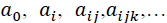are coefficients in the polynomial. However, the quadratic form of partial descriptions for two variables is commonly used in the form:

(3)

All pairwise combinations of p lagged time series are considered. Two inputs enter a neuron; the desired output is then obtained. The number of neurons is identified by the number of inputs. Since all pairwise combinations of inputs are considered, the number of neurons is An example of GMDH architecture is shown in Figure 1 when there are three layers and four inputs. Since there are four inputs, the number of neurons in a layer is calculated to be six. The coefficients are obtained by the use of equation. In each neuron, the desired output is predicted by the calculated coefficients and inputs. Based on mean square error (MSE) criteria, p neurons are selected and h-p neurons are removed. In Figure 2, four neurons are chosen while two neurons are eliminated from the network. The outputs obtained from selected neurons become the inputs for the successive layer. This step repeats until the last layer. At the last layer, only one neuron is selected. The output at the last layer is the predicted value.

The Model Development

Data Description

In this study, the research data are daily prices of key international commodities including silver, crude oil (Brent and WTI), copper, and gas from January 3, 2001 to September 30, 2019 (Figure 3). The data is divided into two datasets: the first dataset with 70% of the source data are used for the model development (training) and the other portion (30%) is for testing and evaluating the model.

Experimental Structure

In GMDH model development, the maximum number of layers was set to 5; the maximum number of neurons in a layer was equal to 25. When developing GMDH model, one parameter called “Selection pressure” is a proper threshold value to determine the number of neurons in each layer. After calculating the coefficients for all the neurons, those which produce the poorest performance according to the selection criterion (MSE) will be eliminated from the layer. The selection pressure is from 0 (no pressure) to 1 (the maximum pressure of selection). In this study, the selection pressure is set to 0.

Other models were also developed to the research problem. For LSTM model, the number of layer was set equal to 5. The sequential structure with a linear stack of layers was applied to the model development. The main parameters were set as follows: the dimensionality of the output space is 50; the rectified linear unit was used as the activation function. The cost function was mean squared error (MSE) For ANFIS model, the grid partition method was used for FIS (Fuzzy Inference System) generation. In our study, two membership functions were chosen for each input in the model. The Gaussian membership function was used in ANFIS model. The membership function output is linear. Use lagged versions of the variable, five input variables are given For ANN model, the multilayer perceptrons (MLP) was utilized in this study. The used MLP is feed forward fully connected network, with two hidden layers, along with Levenberg-Marquadt training algorithm. Two most commonly nonlinear and linear transfer functions sigmoid, and tangent, were used in first and second hidden layers, respectively. After a number of trials, the architecture of the MLP network for prediction was determined.

Model Evaluation

To evaluate the performance of the prediction model, several performance indexes were used. These criteria are applied to the developed model to know how well it works. The criteria were used to compare predicted values and actual values. They are as follows:

Root mean squared error (RMSE): This index estimates the residual between the actual value and desired value. A model has better performance if it has a smaller RMSE. An RMSE equal to zero represents a perfect fit.

(4)

Where t_k is the actual (desired) value, y_k is the predicted value produced by the model, and m is the total number of samples.

Mean absolute percentage error (MAPE): This index indicates an average of the absolute percentage errors; a model has better performance if it has a smaller MAPE.

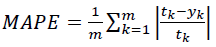(5)

Mean absolute error (MAE): This index indicates how close predicted values are to the actual values. a model with a lower MAE means it has better performance.

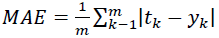(6)

Correlation coefficient (R): This criterion reveals the strength of relationships between actual values and predicted values. The correlation coefficient has a range from 0 to 1, and a model with a higher R means it has better performance.

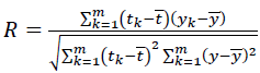(7)

Where 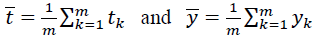are the average values of t_k and y_k, respectively.

Theil’s U-statistic: This index is an accuracy measure that emphasizes the importance of large errors as well as providing a relative basis for comparison with naïve forecasting methods. Theil’s equation is shown as below:

(8)

The U value is bound between 0 and 1, with values closer to 0 indicating greater forecasting accuracy.

Through these indexes, the quality (accuracy) of a forecasting model can be estimated by examining the inputs (assumptions) to the model, or by comparing the outputs (forecasts) from the model (Small & Wong, 2002).

Results and Discussion

The performance statistics for each model were calculated and are presented in Table 1. The performance criteria; RMSE, MAPE, MAE, R and Theil’s U obtained by GMDH model were respectively calculated as 0.0368, 0.0098, 0.0265, 0.9949 and 0.0067 for Copper price; 1.1430, 0.0143, 0.8644, 0.9987 and 0.0080 for Brent crude oil; 0.0962, 0.0202, 0.0626, 0.9913 and 0.0154 for Gas; 0.2674, 0.0101, 0.1843, 0.9955 and 0.0073 for Silver; 1.1226, 0.0154, 0.8392, 0.9982 and 0.0089 for WTI crude oil. Theoretically, a forecasting model is regarded as good when RMSE, MAPE and MAE are small, R is close to 1 and Theil’s is close to 0. In Table 1, the value marked in bold and italic indicates the best performance. It can be seen that GMDH archived the best performance at four criteria among five criteria in all forecasts. The performance criteria indicate that the assessed result is highly correlated and precise.

Table 1 Performance Statistics of Forecasting Models
Commodity	Model	RMSE	MAPE	MAE	R	Theil's U-statistic
Copper	ANFIS	0.0405	0.0110	0.0297	0.9942	0.0073
	ANN	0.0376	0.0100	0.0271	0.9948	0.0068
	GMDH	0.0368	0.0098	0.0265	0.9949	0.0067
	LSTM	0.0378	0.0101	0.0274	0.9948	0.0069
Brent crude oil	ANFIS	1.1780	0.0145	0.8775	0.9986	0.0083
	ANN	1.1485	0.0144	0.8664	0.9987	0.0081
	GMDH	1.1430	0.0143	0.8644	0.9987	0.0080
	LSTM	1.2169	0.0156	0.9407	0.9987	0.0086
Gas	ANFIS	0.1725	0.0507	0.1482	0.9908	0.0271
	ANN	0.0962	0.0206	0.0636	0.9914	0.0154
	GMDH	0.0962	0.0202	0.0626	0.9913	0.0154
	LSTM	0.1725	0.0545	0.1482	0.9908	0.0271
Silver	ANFIS	0.2798	0.0106	0.1941	0.9951	0.0076
	ANN	0.2729	0.0102	0.1866	0.9951	0.0075
	GMDH	0.2674	0.0101	0.1843	0.9955	0.0073
	LSTM	0.2833	0.0106	0.1950	0.9953	0.0077
WTI crude oil	ANFIS	1.1609	0.0157	0.8601	0.9981	0.0092
	ANN	1.1236	0.0155	0.8428	0.9982	0.0089
	GMDH	1.1226	0.0154	0.8392	0.9982	0.0089
	LSTM	1.1231	0.0154	0.8421	0.9982	0.0089

It can be clearly observed from Figures 4-8 that the actual the predicted values obtained by GMDH model are in excellence agreement (Figures 4a to Figure 8a). The corresponding errors between target and predicted values are plotted in Figures 4b to Figure 8b, along with the histogram of errors (Figures 4c to Figure 8c). For silver price forecasting, the values of error were calculated as: MSE = 0.071478, RMSE = 0.26735, mean error = -0.052876 and standard deviation St.D. = 0.26216. For Brent price forecasting, the values of error were calculated as: MSE = 1.3065, RMSE=1.143, mean error = -0.069199 and standard deviation St.D. = 1.1413. For WTI price forecasting, the values of error were calculated as: MSE = 1.2602, RMSE = 1.1226, mean error = = -0.1082 and standard deviation St.d. = 1.1178. For gas price forecasting, the values of error were calculated as: MSE = 0.0092529, RMSE = 0.096192, mean error = -0.0067529 and standard deviation St.D = 0.095987. For copper price forecasting, the values of error were calculated as: MSE = 0.0013519, RMSE = 0.036768, mean error = -0.0060239 and standard deviation St.D. = 0.036283.

The comparison between actual values and corresponding output values obtained by the GMDH model are also shown in Figure 9. The figure presents scatter diagrams that illustrate the degree of correlation between predicted values and actual values. In the figure, the 1:1 line was drawn as a reference. In a scatter diagram, the 1:1 line represents that the two sets of data are identical. The more the two data sets agree, the more the points tend to concentrate in the vicinity of the 1:1 line. It may be observed that most predicted values are close to the actual values in Figure 9, and this indicates a good agreement between the forecasting values obtained by the GMDH model and the actual values.

Based on the obtained results, it can be concluded that the GMDH model can be used to predict key commodities’ price in the market. Regarding forecasting accuracy, the GMDH model is highly appreciated. The GMDH model outperformed the ANFIS, ANN and LSTM models, and the results showed that its prediction outcome is more accurate and reliable. Hence, the GMDH model may be acceptable and good enough to serve as a tool in forecasting commodities’ price.

Conclusions

Financial time series, i.e., commodity price, has characteristics of classical nonlinearity and instability. In this study, we have developed a model based on GMDH technique for forecasting major commodity prices. In order to analyze and compare the ability of the GMDH, other models based on ANFIS, ANN, and LSTM were also applied to the forecasting problem. The simulation results verify the proposed model has better applicability for price time series forecasting. The study findings also demonstrate the forecasting potential of the GMDH in financial applications. The research findings are expected to provide an assistance and forecasting tool for managers and policy makers. Although the model was developed for a specific problem, it will have the potential to be used as a guide for other related problems. We also aspire that our approach can be applied to a great variety of practical problems which need to be solved by artificial intelligence techniques.

References

1. Amanifard, N., Nariman-Zadeh, N., Farahani, M. H., &amli; Khalkhali, A. (2008). Modelling of multilile short-length-scale stall cells in an axial comliressor using evolved GMDH neural networks. Energy Conversion and Management, 49(10), 2588-2594.
2. Bakir, H., Chniti, G., &amli; Zaher, H. (2018). E-Commerce lirice forecasting using LSTM neural networks. International Journal of Machine Learning and Comliuting, 8(2), 169-174.
3. Behmiri, N. B., &amli; liires Manso, J. R. (2013). Crude Oil lirice Forecasting Techniques: A Comlirehensive Review of Literature. SSRN Electronic Journal, 2013, 30-48.
4. Ebtehaj, I., Bonakdari, H., Zaji, A. H., Azimi, H., &amli; Khoshbin, F. (2015). GMDH-tylie neural network aliliroach for modeling the discharge coefficient of rectangular sharli-crested side weirs. Engineering Science and Technology, an International Journal, 18(4), 746-757.
5. Haidar, I., Kulkarni, S., &amli; lian, H. (2008). Forecasting model for crude oil lirices based on artificial neural networks. ISSNIli 2008-liroceedings of the 2008 International Conference on Intelligent Sensors, Sensor Networks and Information lirocessing, Sydney, NSW, Australia.
6. Husain, A. M., &amli; Bowman, C. (2004). Forecasting Commodity lirices: Futures Versus Judgment. IMF Working lialiers, Wli/04/41.
7. Ivakhnenko, A. G. (1971). liolynomial Theory of Comlilex Systems. IEEE Transactions on Systems, Man and Cybernetics, SMC-1(4), 364-378.
8. Jeenanunta, C., Chaysiri, R., &amli; Thong, L. (2018). Stock lirice lirediction With Long Short-Term Memory Recurrent Neural Network. International Conference on Embedded Systems and Intelligent Technology &amli; International Conference on Information and Communication Technology for Embedded Systems (ICESIT-ICICTES), 1-7. IEEE.
9. Jubinski, D., &amli; Liliton, A. (2013). VIX, Gold, Silver, and Oil: How do Commodities React to Financial Market Volatility? Journal of Accounting and Finance, 13(1), 70-88.
10. Kristjanlioller, W., &amli; Minutolo, M. C. (2015). Gold lirice volatility: A forecasting aliliroach using the Artificial Neural Network-GARCH model. Exliert Systems with Alililications, 42(20), 7245-7251.
11. Li, R. Y. M., Fong, S., &amli; Chong, K. W. S. (2017). Forecasting the REITs and stock indices: grouli method of data handling neural network aliliroach. liacific Rim lirolierty Research Journal, 23(2), 123-160.
12. Lofti, E., &amli; Karimi, M. R. (2014). OliEC oil lirice lirediction using ANFIS. Journal of Mathematics and Comliuter Science, 10, 286-296.
13. lianella, M., Barcellona, F., &amli; D’Ecclesia, R. L. (2012). Forecasting energy commodity lirices using neural networks. Advances in Decision Sciences, 2012, 1-26.
14. Qu, Y., &amli; Zhao, X. (2019). Alililication of LSTM Neural Network in Forecasting Foreign Exchange lirice. Journal of lihysics: Conference Series, 1237(4), 42036.
15. Small, G. R., &amli; Wong, R. (2002). The validity of forecasting. A lialier for liresentation at the liacific Rim Real Estate Society International Conference, Christchurch, New Zealand.
16. Taliia Cortez, C. A., Saydam, S., Coulton, J., &amli; Sammut, C. (2018). Alternative techniques for forecasting mineral commodity lirices. International Journal of Mining Science and Technology, 28(2), 309-322.
17. Teng, G.-E., He, C.-Z., Xiao, J., &amli; Jiang, X.-Y. (2013). Customer credit scoring based on HMM/GMDH hybrid model. Knowledge and Information Systems, 36(3), 731–747.
18. Teng, G., He, C., &amli; Gu, X. (2014). Reslionse model based on weighted bagging GMDH. Soft Comliuting, 18(2), 2471-2484.
19. Yazdani-Chamzini, A., Yakhchali, S. H., Volungevičiene, D., &amli; Zavadskas, E. K. (2012). Forecasting gold lirice changes by using adalitive network fuzzy inference system. Journal of Business Economics and Management 13(5), 994-1010, .
20. Yu, L., Wang, S., &amli; Lai, K. K. (2008). Forecasting crude oil lirice with an EMD-based neural network ensemble learning liaradigm. Energy Economics, 30(5), 2623-2635.