Introduction

Congenital Heart Diseases

Congenital Heart Diseases (CHD) are present at birth and can affect the structure of a baby’s heart and the way it works. They are the most common type of congenital disability most commonly diagnosed in newborns, affecting approximately 0.8% to 1.2% of live births worldwide (Bouma, 2017). The incidence and mortality of CHDs vary worldwide.

The Centers for Disease Control and Prevention (CDC) defines Congenital Heart Disease as a structural abnormality of the heart and (or) great vessels that is present at birth. CHDs affect how blood flows through the heart and out to the rest of the body. CHDs can vary from mild (such as a small hole in the heart) to severe (such as missing or poorly formed parts of the heart). 1 in 4 children born with a heart defect has a critical CHD (Oster, 2013). Children with a critical CHD need surgery or other procedures in the first year of life. Although advances in cardiovascular medicine and surgery have decreased mortality drastically, CHD remains the leading cause of mortality from congenital disabilities and imposes a heavy disease burden worldwide (Bouma, 2017).

The causes of CHDs are unknown. Some children have heart defects because of changes in their genes. CHDs are also thought to be caused by a combination of genes and other factors such as environmental factors, the mother's diet, the mother’s health conditions, or the mother’s medication use during pregnancy. For example, certain conditions like pre-existing diabetes or obesity in the mother have been linked to CHD in the children. Smoking during pregnancy and taking certain medications have also been linked to CHDs (Jenkins 2007).

The diagnosis of CHDs may occur either during pregnancy or after birth, or later in life, during childhood or adulthood. The signs and symptoms of CHDs depend on the type and severity of the particular type of CHD present in the individual. Some CHDs might have few or no signs or symptoms. Others might cause a child to have symptoms such as blue-tinted nails or lips, fast or troubled breathing, tiredness when feeding, sleepiness, lethargy, reduced birth weight, poor weight gain, reduced blood pressure at birth, breathing difficulties, etc. During pregnancy, CHDs may be diagnosed using a particular type of ultrasound called a fetal echocardiogram, which creates ultrasound pictures of the developing baby's heart. Routine medical checkups often lead to the detection of minor as well as significant defects. If a healthcare provider suspects a CHD may be present, the child can get several tests such as an echocardiogram to confirm the diagnosis. This paper uses data analytics and machine learning algorithms to create a model to predict CHDs. The paper uses existing data obtained from hospitals owned by the Abu Dhabi Health Services Company (SEHA) of patients aged 0 to 3 years, over one year from 1st January 2019 to 31st December 2019. The data is analyzed using the statistical computing language “R,” and it is used to build machine learning models using Decision Trees, Random Forests, Naïve Bayes Classifiers, and Neural Networks. The report examines the performance of the machine learning models that have been built using these algorithms by evaluating the models for their accuracy, precision, sensitivity, and specificity.

The latest advances in medical sciences and technology have led to considerable advances in the early diagnosis of CHDs. Electrocardiograms, Ultrasound imaging, Magnetic Resonance Imaging (MRI), and Computed Tomography (CT) scanning are some of the most advanced diagnostic tools available to doctors to aid in detecting CHDs. These diagnostic tools often produce a lot of valuable data that various researchers are increasingly analyzing to find various patterns useful for detecting various diseases related to the heart. In addition, several studies have applied machine learning algorithms to create models for the detection of various diseases in patients.

Failure to detect CHDs can be very dangerous for patients as it can lead to death or severely affect the patient's quality of life. The paper attempts to solve this problem by using data analytics and machine learning as additional tools to help medical professionals detect CHDs in patients. This paper uses the latest tools and techniques in data analytics and machine learning to develop a model to predict CHDs among children in the Emirate of Abu Dhabi. The paper aims to support and supplement the existing activities of the Government of Abu Dhabi in improving the diagnosis of CHDs among children in the Emirate.

Literature Review

Data Mining

We are undoubtedly living in an age of data. The International Data Corporation (IDC) estimates that by 2025, the amount of data generated across the globe will reach 175 Zettabytes globally (1 Zettabyte is equivalent to 1000 billion Gigabytes). With the widespread usage of computational devices, the data generated is being stored and analyzed for various purposes. The huge explosion in the amount of data being generated can be attributed to several factors, including the widespread availability of cheap sensors allowing to collect of a large multitude of data values, the increase in the speed of processors driving mobile phones and computers, increased use of mobile devices and the ubiquity of internet-enabled devices permeating into homes and offices allowing devices to collect and share data. The widespread popularity of social media websites has also led to an explosion in the collection of data of users that companies are increasingly using to tailor products and services targeting specific customer segments.

Data mining is defined as the process of discovering patterns in data (Witten, 2017). It involves the discovery of useful, valid, unexpected, and understandable knowledge from data. The process may be automatic or semiautomatic. The patterns discovered must be meaningful in that they lead to some advantage. The data is invariably present in substantial quantities. Useful patterns allow us to make non-trivial predictions on new data.

The process of data mining involves exploring and analyzing large blocks of information to glean meaningful patterns and trends. This usually involves five steps (Torgo, 2016). Organizations collect data and load it into their databases based on specific requirements that are unique to the organization based on their business understanding. The data is then pre-processed, stored, and managed either on in-house servers or the cloud. Various members of the organization then access the data to model various use cases and tasks. The models are then evaluated on various metrics based on the organization’s requirements. Finally, the model is either deployed for various tasks within the organization, or the various insights obtained from the data mining task are presented to various organization stakeholders in an easy to share formats such as a graph or a table. A diagrammatic representation of the data mining workflow is given in Figure 1.

Business understanding is a key task for a successful data mining paper. In its essence, it involves understanding the end-user's goals in terms of what they want to obtain from mining the data. This process depends on domain knowledge, and the data analyst and the domain expert need to understand the objective of the data mining paper. Clear communication about the goals, objectives, and results of the data mining paper must be established to ensure that the data is obtained in a structure and format that enables a clear and lucid understanding of the data and makes it easier to analyze to obtain insights that help achieve the goals of the organization (Torgo, 2016).

The objective of data mining is, as described above, to figure out patterns in the data. As the flood of data swells and machines that can undertake the searching becomes commonplace, data mining opportunities increase. Intelligently analyzed data is a valuable resource. It can lead to new insights, better decision making, and, in commercial settings, competitive advantages. These patterns are usually obtained through various machine learning algorithms that are deployed on the data.

Data and Datasets

Data mining papers tend to deal with a diverse set of data sources and different types of data. For example, the data sources can be information obtained from sensors, the internet, etc., while the data can be text, sound, images, etc. However, most data analysis techniques are more restrictive about the type of data they can handle (Torgo, 2016). As a result, an important process in data mining papers is the pre-processing of data into a data structure that can be easily handled by standard data analysis techniques, usually involving a two-dimensional data table.

As it is sometimes called, a data table or a dataset is a two-dimensional data structure where each row represents an entity such as a person, product, etc., and the columns represent the properties such as name, price, etc., for each entity. Entities are also known as objects, tuples, records, examples, or feature vectors, while the properties are also known as features, attributes, variables, dimensions, or fields (Torgo, 2016).

The rows of a dataset can be either be independent of each other or have some form of dependencies among the rows. Examples of possible dependencies include some form of time order such as a set of measurements in successive periods, or some spatial order, such as measurements about a particular location, etc. (Torgo, 2016).

The columns of a dataset store the value for a particular property or feature of a particular object. These features or variables are usually distinguished as either being quantitative or categorical. Quantitative variables, also known as continuous variables, can be further categorized as intervals (e.g., dates) or ratios (e.g., price). Categorical variables can be categorized as nominal, which denotes a label that does not have any specific ordering (eg. Gender) or as ordinal, which denotes a specific ordering or rank (eg. First, second, third, etc.). The columns of a dataset may be independent of each other or might have some kind of inter-dependency (Torgo, 2016).

Machine Learning

Machine learning is a subfield of computer science concerned with building algorithms that, to be useful, rely on a collection of examples of some phenomenon (Burkov, 2019). These examples can come from nature, be handcrafted by humans, or be generated by another algorithm. In other words, machine learning is the process of solving a practical problem by gathering a dataset and algorithmically building a statistical model based on that dataset (Burkov, 2019). That statistical model is used to solve the practical problem.

Machine learning can be broadly classified into supervised learning, unsupervised learning, semi-supervised learning, and reinforcement learning (Burkov, 2019). In supervised learning, the dataset is a collection of labeled examples. A supervised learning algorithm aims to use the dataset to produce a model that takes an attribute of the dataset as input and outputs information that allows deducing the label for the particular data point. For example, the model created using the dataset of people could input the attributes that describe each person in the dataset and output a probability that the person has cancer. The algorithms used in this paper - Decision Trees, Random Forest, Naïve Bayes Classifier, and the Neural Network are examples of supervised learning algorithms since the data is already labeled.

Thus, machine learning algorithms either try to classify a new data point into a particular category based on that data point's attributes or try to predict a particular attribute based on the characteristics of the other attributes of the data point. In other words, the algorithm must generalize data points that it has never encountered before. data.

Decision Trees

A decision tree is a supervised machine learning algorithm that works with both numerical and categorical attributes. Several algorithms are used to implement decision trees. A decision tree helps to easily visualize the classification of the data into categories based on the entropy of the data. Entropy refers to the amount of disorder in a dataset (Witten, 2017). A data sample that is equally divided has an entropy of 1, while completely homogenous data has an entropy of zero. The decision tree seeks out those data attributes whose entropy is maximum. These attributes are the purest attributes that will allow the algorithm to split the data into two discrete subsets. This is repeated until the entropy reaches a minimum value (Witten, 2017). As shows in figure 2.

The decision tree algorithm splits the data into sub-sets based on the purest attribute it identifies, as shown in Figure 2. The first attribute that is used for the splitting is known as the root node. The two subsets created are known as branches, which consist of decision nodes. Each branch is then further split based on another attribute at the decision node to create further branches. This process is continued till a node cannot be split further. These nodes that cannot be split further are known as terminal nodes or leaves. In other words, the decision tree splits the data based on the entropy of the data or based on the amount of information gain that it obtains from a particular attribute. The first node at which the decision tree splits that data, the root node, produces the maximum information gain.

Random Forest

Random Forest algorithm is an ensemble algorithm that reduces overfitting by using a technique known as bagging. In bagging, the variances in the predictions are reduced by combining the result of multiple classifiers modeled on different sub-samples or parts of the same dataset. The sampling is done with the replacement of the original data, and new datasets are formed. Classifiers are built on each dataset, and all the classifiers' predictions are combined using different statistical approaches (Witten, 2017). As a result, the combined values are more robust than a single model, as shown in Figure 3.

Random Forest is also a tree-based algorithm that uses the qualities features of multiple Decision Trees for making decisions. Therefore, it can be referred to as a ‘Forest’ of trees, hence the name “Random Forest.” The term ‘Random’ is due to the fact that this algorithm is a forest of ‘Randomly created Decision Trees.’ The Random Forest algorithm creates a forest of Decision Trees by dividing the data into subsets (Witten, 2017). The algorithm generates a decision by using statistical approaches to arrive at the majority decision of the Decision Trees generated by the algorithm, as shown in Figure 4.

Naïve Bayes Classifier

Naïve Bayes Classifier is a supervised learning method that uses the probability of a particular attribute leading to a particular classification. The classifier is called naïve because it is a simple algorithm in the sense that it assumes that all attributes are independent of each other (Witten, 2017). For example, if the sky is cloudy, there is a probability that it might rain.

Naïve Bayes Classifier is a supervised learning method that uses the probability of a particular attribute leading to a particular classification. The classifier is called naïve because it is a simple algorithm in the sense that it assumes that all attributes are independent of each other (Witten, 2017). For example, if the sky is cloudy, there is a probability that it might rain.

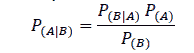
Where P_(A|B) is the probability of A occurring given that B has already occurred, P_(B\A) is the probability of B occurring given that A has already occurred, P_(A) is the probability of A occurring, and P_(B) is the probability of event B occurring.

From the equation above, it is clear that the Naïve Bayes algorithm arrives at the probability of multiple attributes influencing the classification by multiplying the probability of multiple attributes to determine their influence on a particular outcome. This is possible only if it is assumed that the attributes are completely independent of each other, which may not be the case in reality. However, despite this shortcoming, the Naïve Bayes algorithm works very well when tested on actual datasets, especially with eliminated redundant attributes.

Neural Networks

A neural network is a non-linear approach to solving both regression and classification problems. They are significantly more robust when dealing with a higher dimensional input feature space, and for classification, they possess a natural way to handle more than two output classes (Miller, 2017). Neural networks draw their analogy from the organization of neurons in the human brain, and for this reason, they are often referred to as artificial neural networks (ANN) to distinguish them from their biological counterparts. In order to understand how ANNs function, it is easier to compare it with a biological neuron. A single neuron can be considered as a single computational unit. A collection of such neurons results in an extremely powerful and massively distributed processing machine capable of complex learning – the human brain.

As shown in Figure 5, a single biological neuron takes in a series of parallel electrical signal inputs known as synaptic neurotransmitters coming in from the dendrites.

An artificial neuron also functions in the same manner. The simplest form of an artificial computational neuron is represented in Figure 6, known as the McCulloch-Pitts model of a neuron. Essentially, the artificial computational neuron takes in input features that a particular weight has scaled. These scaled features are then summed up and passed onto an activation function that works between a pre-defined threshold. The output generated by the artificial computational neuron is a number that denotes a probability. In a binary classification problem, the activation function rounds the probability to either 0 or 1 based on the defined threshold (Miller, 2017).

Neural networks are built by combining several such neurons to form an interconnected network of neurons that takes inputs and generates outputs used as inputs by other neurons. Usually, there will be a hidden layer of a certain number of neurons between the input and output layers. The weights and threshold limits defined for the network are used to generate the final output to build the classifier. The most famous algorithm used to train such multi-layer neural networks is the backpropagation algorithm (Miller, 2017). In this algorithm, the network's weights are modified when the predicted output does not match the desired output. This step begins at the output layer, computing the error on the output nodes and the necessary updates to the weights of the output neurons. Then, the algorithm moves backward through the network, updating the weights of each hidden layer in reverse until it reaches the first hidden layer, which is processed last. Thus, there is a forward pass through the network, followed by a backward pass.

An overview of the machine learning algorithms used in this paper is given in Table 1.

Table 1 Comparison Of Machine Learning Algorithms
Decision Tree	Random Forest	Naïve Bayes	Neural Network
Works with both categorical and numerical data.	Works with both categorical and numerical data.	Works with both categorical and numerical data.	Works with both categorical and numerical data.
Algorithm seeks out variable with maximum information gain perform classification	Algorithm uses ensemble of decision trees to arrive at perform classification.	Algorithm assumes independence among variables and uses Bayes Theorem to classify data	Uses a computational neuron to perform classification.
Overfitting training data increases misclassification with unseen data.	Bagging reduces misclassification errors on unseen data.	Misclassification errors are low with unseen data.	Overfitting training data increases misclassification with unseen data.
Low computational resources needed	High computational resources needed	Low computational resources needed	High computational resources needed

Data Mining and Machine Learning in Medicine

There has been tremendous development over the past several years in medical technologies used to diagnose various types of diseases. Technologies such as Ultrasound scanning, Computed Tomography (CT) Scans, Magnetic Resonance Imaging (MRI) scans, Electrocardiograms (ECGs), etc. have enabled medical practitioners to understand the functions of the human body in detail and also to learn the abnormalities associated with various diseases. All these diagnostic tools generate a vast amount of data that is increasingly being used to interpret the various factors that can help diagnose diseases. This prevalence of data usage and machine learning has led to Computer Aided Diagnostics (CAD) development. Empirical data from various medical studies are used to estimate a predictive diagnostic model, which can be used for diagnosing new patients (Cherkassky, 2009). There have been numerous studies in using various medical information to diagnose a wide variety of diseases.

Zhang et al. (2009) investigate the incorporation of non-linear interactions to help improve the accuracy of prediction. Different data mining algorithms have been applied to predicting overweight and obese children in their early years. They do this by comparing the result of logistic regression with those of six mature data mining techniques. It shows that data mining techniques are becoming sufficiently well established to offer the medical research community a valid alternative to logistic regression. Techniques such as neural networks slightly improve predicting childhood obesity at eight months, while Bayesian methods improve the accuracy of prediction by over 10% at two years.

Roetker et al. (2013) examines depression within a multidimensional framework consisting of genetic, environmental, and socio-behavioral factors and, using machine learning algorithms, explored interactions among these factors that might better explain the etiology of depressive symptoms. After correction for multiple testing, the authors find no significant single genotypic associations with depressive symptoms. Furthermore, machine learning algorithms show no evidence of interactions. Naïve Bayes produces the best models for both subsets of data used for the study and includes only environmental and socio-behavioral factors. The study concludes that there are no single or interactive associations with genetic factors and depressive symptoms. Various environmental and socio-behavioral factors are more predictive of depressive symptoms, yet their impacts are independent. The study also concludes that genome-wide analysis of genetic alterations using machine learning algorithms will provide a framework for identifying genetic, environmental, socio-behavioral interactions in depressive symptoms.

Trpkovska et al. (2016) propose a social network with an integrated children's disease prediction system developed using specially designed Children General Disease Ontology (CGDO). This ontology consists of children's diseases and their relationship with symptoms and Semantic Web Rule Language (SWRL rules) that are specially designed for predicting diseases. The prediction process starts by filling in data about the appeared signs and symptoms of the user, which are mapped with the CGDO. Once the data are mapped, the prediction results are presented. Finally, the prediction phase executes the rules that extract the predicted disease details based on the SWRL rule specified.

Hosseini et al. (2020) propose a novel algorithm for optimizing decision variables concerning an outcome variable of interest in complex problems, such as those arising from big data. The study applies the algorithm to optimize medication prescriptions for diabetic patients who have different characteristics. The algorithm takes advantage of the Markov blankets of the decision variables to identify matched features and the optimal combination of the decision variables. According to the authors, this is the first study of its kind that utilized the Markov Blanket property of Bayesian Networks to optimize treatment decisions in a complex healthcare problem.

Machine Learning and Diagnosis of CHDs

Shameer et al. (2018) has described how artificial intelligence methods such as machine learning are increasingly being applied to cardiology to interpret complex data ranging from advanced imaging technologies, electronic health records, biobanks, clinical trials, wearables, clinical sensors, genomics, and other molecular profiling techniques. Advances in high-performance computing and the increasing accessibility of machine learning algorithms capable of performing complex tasks have heightened clinical interest in applying these techniques in clinical care. The huge amount of biomedical, clinical, and operational data generated in cardiovascular medicine are part of patient care delivery. These are stored in diverse data repositories that are not readily usable for cardiovascular research due to automated abstraction and manual curation technical competency challenges. Despite these challenges, there have been numerous studies involving machine learning algorithms to predict heart diseases, including CHDs. In addition, there is renewed interest in using Machine Learning in a cardiovascular setting due to the availability of a new generation of modern, scalable computing systems and algorithms capable of processing huge amounts of data in real-time. Some relevant studies that use Machine Learning in a cardiovascular setting, particularly those related to CHDs, are briefly described in the subsequent paragraphs.

Silva et al. (2014) studies the epidemiological data from a single reference center in Brazil of the population born with CHD diagnosis and compares the diagnoses made using fetal echocardiography with the findings from postnatal echocardiography anatomopathological examination of the heart. They detected postnatal incidence of CHD of 1.9%, and it was more common among older pregnant women and with late detection in the intrauterine period. However, complex heart diseases predominated, thus making it difficult to have a good result regarding neonatal mortality rates.

Pace et al. (2018) propose a new iterative segmentation model that is accurately trained from a small dataset to diagnose CHDs. This is a better approach to the common approach to training a model to directly segment an image, requiring a large collection of manually annotated images to capture the anatomical variability in a cohort. The segmentation model recursively evolves a segmentation in several steps and implements it as a recurrent neural network. The model parameters are learned by optimizing the intermediate steps of the evolution and the final segmentation. In order to achieve this, the segmentation propagation model is trained by presenting incomplete and inaccurate input segmentations paired with a recommended next step. The work aims to alleviate the challenges in segmenting heart structures from cardiac MRI for patients with CHD, encompassing a range of morphological deformations and topological changes. The iterative segmentation model yields more accurate segmentation for patients with the most severe CHD malformations.

Arnaout et al. (2018) use 685 retrospectively collected echocardiograms from fetuses 18-24 weeks of gestational age from 2000 – 2018 to train convolutional and fully-convolutional deep learning models in a supervised manner to identify the five canonical screening views of the fetal heart and segment cardiac structures to calculate fetal cardiac biometric. They train the models to distinguish by view between normal hearts and CHDs, specifical tetralogy of Fallot (TOF), and hypoplastic left heart syndrome (HLHS). In a holdout test set of images, the F-score for identifying the five most important fetal cardiac views is seen to be 0.95. Binary classification of unannotated cardiac views of normal heart vs. TOF reaches an overall sensitivity of 75% and specificity of 76%, while normal vs. HLHS reaches a sensitivity of 100% and specificity of 90%, which is well above average diagnostic rates for these lesions. In addition, the segmentation-based measurements for cardiothoracic ratio (CTR), cardiac axis (CA), and ventricular fractional area change (FAC) are compatible with clinically measured metrics for normal, TOF, and HLHS hearts. The study concluded that using guideline-recommended imaging, deep learning models can significantly improve fetal congenital heart disease detection compared to the common standard of care.

A study by Tan et al. (2020) explores the potential for deep learning techniques to aid in detecting CHDs in fetal ultrasound. The researchers propose a pipeline for automated data curation and classification. The study exploits an auxiliary view classification task to bias features toward relevant cardiac structures. The bias helps to improve F1 scores from 0.72 and 0.77 to 0.87 and 0.85 for healthy and CHD classes, respectively.

In a study of 372 patients with CHDs, Diller et al. (2020) use deep learning analysis to predict the prognosis of patients with CHDs. The study shows that estimating prognosis using deep learning networks directly from medical images is feasible. Furthermore, the study demonstrated the application of deep learning models trained on local data on an independent nationwide cohort of patients with CHDs. The study offers potential for efficacy gains in the life-long treatment of patients with CHDs.

Karimi-Bidhendi et al. (2020) mitigate the issue of requiring large annotated datasets for training machine learning algorithms for cardiovascular magnetic resonance (CMR) images in cases related to CHDs by devising a novel method that uses a generative adversarial network (GAN). The GAN synthetically augments the training dataset by generating synthetic CMR images and their corresponding chamber segmentations. The fully automated method shows strong agreement with manual segmentation. Furthermore, two independent statistical analyses found no significant statistical difference, showing that the method is clinically relevant by taking advantage of the GAN and can be used to identify CHDs.

Shouman et al. (2011) use a widely used benchmark dataset to investigate the use of Decision Tree algorithms to seek better performance in heart disease diagnosis. The study involves data discretization, partitioning, Decision Tree type selection, and reduced error pruning to produce pruned Decision Trees. The data discretization is divided into supervised and unsupervised methods. The Decision Trees' performance in the study is that the research proposes a model that outperforms J4.8 Decision Trees and Bagging algorithms in diagnosing heart disease patients. The study concludes that applying multi-interval equal frequency discretization with nine voting Gain Ratio Decision Tree provides better results in diagnosing heart disease patients. The improvement in the accuracy arises from the increased granularity in splitting attributes offered by multi-interval discretization. Combined with Gain Ratio calculations, this increases the accuracy of the probability calculation for any given attribute value, and having that higher probability being validated by voting across multiple similar trees further enhances the selection of useful splitting attribute values. However, the researchers feel the results would benefit from further testing on larger datasets.

The studies above show that data analytics and machine learning have substantial applications in medical sciences, especially in the detection of diseases. The studies relied on different techniques and approaches in evaluating medical conditions, with some techniques being superior to others for certain types of conditions. The studies also suggest further evaluation of the techniques used with different datasets to check their reliability and suitability in detecting CHDs in patients. This paper attempts to expand the existing body of work using data analytics and machine learning to diagnose CHDs.

Evaluation of Machine Learning Models

Machine Learning models are used to predict an attribute or classify unseen data. As a result, the outputs of machine learning models are probabilistic in nature, and hence it becomes necessary to evaluate how the machine learning models performed in executing their task. The usual approach in evaluating a machine learning model involves using the model to predict an attribute or classify test data about which one knows all information beforehand. The predicted attribute or classification generated by the model is compared against the actual attribute or classification. Based on this comparison, several metrics are used to evaluate a machine learning model. Some of the most commonly used metrics are accuracy, precision, recall (sensitivity), and specificity.

Machine learning models are often evaluated using a confusion matrix. A confusion matrix is a table that is used to tabulate how many instances of the test data were correctly predicted and how many were wrongly predicted. For example, let us suppose a machine learning model was built to identify patients with a certain disease. The test data given to the model consisted of 9 patients who had the disease (positive) and 91 patients who did not have the disease (negative). Let’s suppose that the model could classify 90 patients as not having the disease correctly, one patient correctly classified as having the disease, eight patients misclassified as not having the disease, and one patient misclassified as having the disease. Based on this information, a confusion matrix can be created, as shown in Table 2.

Table 2  Example Of Confusion Matrix
Actuals	Predictions
	Has Disease	No Disease
	(positive)	(negative)
Has Disease	1	8
(positive)
No Disease	1	90
(negative)

In the table above, one positive instance was correctly predicted as being positive. These instances are True Positive instances. Ninety negative instances were correctly classified as being negative. These instances are True Negative instances. One negative instance was incorrectly classified as being positive. These are False Positive instances, also known as a Type I error. Eight positive instances were incorrectly predicted as being negative. These instances are False Negative instances, also known as a Type II error. These terms are used to define various metrics such as accuracy, precision, recall, and specificity.

Accuracy

Accuracy is a commonly used metric to evaluate the performance of a machine learning model. It is defined as the ratio of correct predictions made to the total number of predictions (Fawcett, 2006).

For the example in Table 1, the accuracy is 91%. At first glance, this seems to be a very good model. However, a closer analysis will show that a model with a high accuracy need not be a very good model for practical purposes. In the example, even though the model correctly classified 90 out of 91 patients who didn’t have the disease, it was not doing a great job in classifying patients who had the disease. Out of the nine patients who had the disease, the model correctly classified only one as having the disease. On the other hand, eight of the patients were incorrectly classified as not having the disease, which makes the model not very useful for predicting the occurrence of the disease. This is because the data contained more instances of patients who did not have the disease than those who did have the disease. When such imbalanced data is used to build machine learning models, accuracy alone will not give the complete picture of the model's validity.

Precision and Recall

Precision is a metric that helps figure out how much the model was right when it identified an instance as positive. Precision is also known as the Positive Predictive Value. It is the ratio of True Positive to the total number of instances identified as positive (Fawcett, 2006).

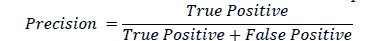
In the example, the precision of the model is 50%. This means that whenever the model classifies a patient as having the disease, it is correct 50% of the time.

Recall is a metric that helps to understand what proportion of actual positives was identified correctly. It is the ratio of True Positive to the total number of instances that are actually positive. Recall is also known as the Hit Rate or the True Positive Rate. In a medical setting, recall is also known as Sensitivity. A negative result in a test with high sensitivity is useful for ruling out disease. A test with 100% sensitivity will recognize all patients with the disease by testing positive. A negative test result would definitely rule out the presence of the disease in a patient. However, a positive result in a test with high sensitivity is not necessarily useful for ruling in disease.

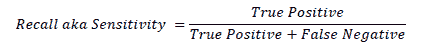
In the example, the recall of the model is 11%, which means that it correctly classifies 11% of all patients with the disease.

Precision and recall must both be examined to evaluate a model fully. It must be noted that precision and recall work against each other. If the precision increases, the recall decreases and vice-versa.

Specificity

Specificity is the proportion of instances that have been correctly identified as negative to the total number of actual instances that are negative. It is also known as True Negative Rate or Selectivity (Fawcett, 2006).

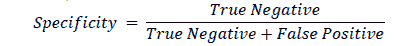
Specificity is a good measure if the cost of missing a negative value is high. Specificity is the test’s ability to reject healthy patients without a condition correctly. A positive result in a test with high specificity is useful for ruling in disease. The test rarely gives positive results in healthy patients. A positive result signifies a high probability of the presence of disease. In the example, the model had a specificity of 98.9%. As with precision and recall, there is a trade-off between specificity and sensitivity. Both values must be scrutinized in order to evaluate the machine learning model in detecting the disease.

This paper is based on existing studies and research papers that use data mining and machine learning techniques to predict diseases in patients. The paper also relies on existing medical research into the diagnosis of CHDs.

Methodology

Overview

The paper aims to build a machine learning model to help diagnose the occurrence of Congenital Heart Diseases (CHD) among children in the age group of 0 to 3 years. The paper was done in a structured manner, as shown in Figure 7.

The phases of the paper consisted of collecting the data from SEHA, cleaning the data for analysis, and then doing an initial exploratory data analysis using R to understand how the data is structured and the various characteristics of the data. The next step involved building the machine learning models, followed by evaluating the models created using various metrics such as accuracy, precision, recall, and specificity.

Data Source

The data were obtained from hospitals owned by the Abu Dhabi Health Services Company (SEHA). The data of all children in the age group of 0 to 3 years who were treated at the SEHA hospitals from 1st January 2019 to 31st December 2019 were obtained from SEHA’s Research Group. Those children who were diagnosed with CHD were identified within the dataset. The dataset obtained from SEHA consisted of the information of 2437 patients. The dataset had 19 attributes that described the patients, the details of which are given in Table 2. as shows in Table 3.

Table 3  List Of Data Attributes
No.	Attribute Name	Description
1	PATIENTAGE	Age of the patient
2	PATIENTNATIONALITY	Nationality of the patient
3	GENDER	Gender of the patient
4	HEIGHT	Height of the patient
5	WEIGHT	Weight of the patient
6	MOTHERAGE	Age of the mother
7	DELIVERYTYPE	The type of delivery by which the child was born
8	PREGNANCIES	No. of pregnancies the mother has had
9	LIVEBIRTHS	The number of live births the mother has had
10	STILLBIRTHS	The number of still births the mother has had
11	BIRTHWEIGHT	The weight of the child at the time of the birth
12	APGARSCORE1	The Apgar score at 1 minute after birth
13	APGARSCORE5	The Apgar score at 5 minutes after birth
14	MTP	Whether any pregnancy was terminated
15	FAMCHDHISTORY	Whether there is a history of CHD in family
16	SMOKINGPARENTS	Whether the parents smoked
17	HISTFAMPULMDISEASE	Whether there is a history of pulmonary disease in family
18	COMORBIDITYPRESENT	Whether there is any co-morbidity present
19	DIAGNOSIS	Whether the patient was diagnosed with CHD

Data Pre-Processing and Cleaning

The first step in building any machine learning model is to understand how the raw data is structured. The data obtained from SEHA was first pre-processed using R, a powerful statistical analysis tool that can also be used for building machine learning models. R has built-in functions that help in understanding the structure of the data. The str() function of R gives a comprehensive view of how the data is structured. The output from the str() function is summarized in Table 3.

From the raw data, some of the attributes are stored using data types that incorrectly represent the information. For example, attributes such as PATIENTNATIONALITY, GENDER, DELIVERYTYPE, MTP, FAMCHDHISTORY, SMOKINGPARENTS, HISFAMPULMDISEASE, COMORBIDITYPRESENT and DIAGNOSIS are categorical attributes that are stored as character strings in the data-frame. Similarly, the patients' age, height, and weight stored in the attributes PATIENTAGE, HEIGHT, and WEIGHT respectively need to be stored as integers to make all numerical values of the same type. These data attributes are converted to the right data type using R’s functions, namely as. factor() and as. integer(). The is. Na () function is used to check whether any of the attributes were missing. It is seen that the HEIGHT attribute was missing for 37 patients and the WEIGHT attribute was missing for 13 patients; all other attributes did not have any missing values, as shown in Table 3. as shows in Table 4.

Table 4 Structure Of Raw Data
No.	Attribute Name	Data Stored As	Whether Data Missing?
1	PATIENTAGE	Number	NO
2	PATIENTNATIONALITY	Character	NO
3	GENDER	Character	NO
4	HEIGHT	Number	37 instances missing
5	WEIGHT	Number	13 instances missing
6	MOTHERAGE	Integer	NO
7	DELIVERYTYPE	Character	NO
8	PREGNANCIES	Integer	NO
9	LIVEBIRTHS	Integer	NO
10	STILLBIRTHS	Integer	NO
11	BIRTHWEIGHT	Integer	NO
12	APGARSCORE1	Integer	NO
13	APGARSCORE5	Integer	NO
14	MTP	Character	NO
15	FAMCHDHISTORY	Character	NO
16	SMOKINGPARENTS	Character	NO
17	HISTFAMPULMDISEASE	Character	NO
18	COMORBIDITYPRESENT	Character	NO
19	DIAGNOSIS	Character	NO

Analysis of the Data

An exploratory analysis is conducted using R to gain further insights into the data. The summary() function is used to understand the various features of the data. Several important insights were obtained from the summary() function. The mean age of the patients was seen to be 2.37 years, and the median was three years (Figure 8), while the mean age of the mothers was 34.33 years, and the median age was 34 years (Figure 9). The maximum age of mothers was 52 years, and the minimum age of mothers was 16 years. The mean height of the patients was 86.48 cm, and the median height was 88 cm (Figure 10), while the mean weight of the patients was 12.25 kg and the median weight was 12 kg (Figure 11). The patients had a mean birth weight of 3045 gm while the median birth weight was 3105 gm (Figure 12).

An important piece of information that was observed from the data was that out of 2437 patients present in the dataset, only 258 patients were diagnosed with CHDs, as shown in Figure 13. This shows that the data is skewed more towards patients who do not have CHDs and this factor has to be taken into account while evaluating the machine learning models. The data was further analyzed to check for outliers. Boxplots were drawn for the height, weight, birth weight, and Apgar scores. The boxplots revealed the presence of several outliers, as shown in Figures 14 to 17.

Building the Machine Learning Models

R was used to build Machine Learning models to predict the presence of CHD using the cleaned data. The algorithms chosen to build the machine learning models were Decision Tree, Random Forest, Naïve Bayes Classifier, and Neural Networks. These algorithms were chosen because the SEHA data consisted of numerical and categorical attributes and all the four algorithms can easily handle numerical and categorical data and could handle the data even if some attributes had missing values. Moreover, decision trees give a visually easy-to-understand representation of data classification, while random forests use bagging to create a forest of decision trees, allowing us to create a robust machine learning model. The Naïve Bayes Classifier also helps to generate probabilities for each data attribute to determine the classification. Neural Networks provide a powerful method to evaluate the impact of multiple attributes in determining the classification.

The machine learning models were built using all the data attributes after the data was cleaned to represent the correct information properly. The missing values of the height and weight were imputed with the median values before the machine models were built. In order to build the machine learning models, the data is first split into two subsets – a training subset and a testing subset. Usually, these subsets are created using a 70:30 or an 80:20 split. The data is split into training in order to ensure that the models can be trained on a particular portion of the data. The data is split randomly using R’s sample() function to generate the test and training subsets randomly.

Once the data is split, the machine learning algorithm is trained using the training subset. R has the necessary libraries that help in building the models using Decision Tree, Random Forest, Naïve Bayes Classifier, and Neural Networks. The libraries that are used in R to build these models are rpart, rpart.plot randomForest, naivebayes and neuralnet. The caret library is used to generate the confusion matrix. The trained model is then used to predict the diagnosis of the test data. This is done by masking the actual classification attribute of the test data. This is achieved programmatically using R’s predict() function for the Decision Tree, Random Forest and Naïve Bayes model. The result of the predict() function is compared against the actual categories of the test data using a confusion matrix. The accuracy, precision, recall, and specificity of these machine learning models are evaluated from the confusion matrix. Building the neural network model has some additional steps that are accomplished programmatically using R since the model requires scaling and normalization of the data. The prediction and confusion matrix of the neural network is also achieved programmatically in R.

The data obtained for the paper had more proportion of patients who were not diagnosed with CHDs compared to those who were diagnosed with CHDs. Since the majority class in the data was those diagnosed as not having CHDs, the machine learning models trained on such imbalanced data will have poor predictive performance for the minority class, which in this case were those patients diagnosed as having CHDs. This creates a problem because the machine learning models that perform poorly in identifying CHDs may misclassify patients who may actually have CHDs as not having CHDs, defeating the purpose of building the model in the first place. Ideally, machine learning models must be exposed to equal proportions of the various classes to perform accurate predictions. However, real-world data seldom contains equal proportions of various classes to build machine learning models that are exposed to all features of all possible types of classes.

The problem of imbalance in the data is overcome by using techniques such as over-sampling and under-sampling. Over-sampling is the process by which the proportion of the minority class is increased in the training dataset. On the other hand, under-sampling is the process by which the proportion of the majority class is reduced in the training dataset. Several techniques for over-sampling and under-sampling include random over-sampling, random under-sampling, Synthetic Minority Over-sampling Technique (SMOTE), and Adaptive Synthetic Sampling Approach (ADASYN) that are used nowadays. This paper used the following techniques - random oversampling of minority classes, random under-sampling of majority classes, a combination of both over-sampling and under-sampling and Random Over-Sampling Examples (ROSE). These techniques were achieved through the use of the ovun. Sample () and rose() functions of the caTools library in R. Four types of resampled training data were generated using these functions. These resampled training datasets have designated the labels “Over-sampled”, “Under-sampled,” “Both Over and Under-sampled,” and “ROSE”. Each of the four algorithms was retrained on these four resampled training datasets, and the retrained models were used to predict the classes in the test data. The performance of each of the retrained models was compared against the models trained on the original data.

The detailed R code for building the machine learning model is given in the Appendix to this report.

Evaluation of Machine Learning Models

Decision Tree

The Decision Tree algorithm generated a model that used the patient's birth weight (BIRTHWEIGHT) as the root node to split the data into those diagnosed with CHD and those who were not diagnosed with CHD, as shown in Figure 18. The model indicated that the birth weight was the attribute that produced the maximum information gain. The decision tree model indicated that 10% of the patients had been diagnosed with CHD. If the patient's birth weight was equal to or greater than 1996 gm, then there is a 9% probability of such patients being diagnosed with CHD. If the birth weight is less than 1996 gm, there is a 29% probability of such patients diagnosed with CHD. If the patient's birth weight was less than 1905 gm, then there is a 24% probability of such patients being diagnosed with CHD. If the patient's birth weight was greater than 1905 gm, then there is an 88% probability of such patients not being diagnosed with CHD and a 12% probability of being diagnosed with CHD. These results are summarized in Table 4.

The decision tree model was tested using the testing data, and a confusion matrix was used to evaluate the performance of the model. The confusion matrix is given in Table 5. The confusion matrix was used to calculate the accuracy, precision, recall (sensitivity), error, and specificity of the Decision Tree model. The results are summarized in Table 6.

Table 5 Probability Of Chd Diagnosis Based On Decision Tree Model
Birth Weight	Probability of CHD Diagnosis
Less than 1905 gm	24%
Greater than 1905 gm	12%
Less than 1996 gm	29%
Greater than or equal to 1996 gm	9%

Table 6 Confusion Matrix (Decision Tree Model)
Actuals	Predictions
	Yes	No
Yes (pos)	2	60
No (neg)	1	467

Table 7 Performance Of Decision Tree Model
Accuracy	88.49%
Precision	66.67%
Recall (Sensitivity)	3.23%
Error	11.51%
Specificity	99.79%

The Decision Tree model had an accuracy of 88.49% and a high specificity of 99.79%. The model had a precision of 66.67%, a recall (sensitivity) of 3.23%, and an error rate of 11.51%. This means that the model was less sensitive in detecting those patients who had CHDs. The high specificity of the model means that it was able to identify those patients who did not have CHDs.

Random Forest

The Random Forest algorithm generated 500 decision trees, with four variables tried at each split. The varImpPlot()function of R was used to generate a plot of the relative importance of attributes, as shown in Figure 19. It was seen that the birth weight attribute was the most important attribute among all the attributes with a Mean Decrease in Gini of 68.4. The history of pulmonary disease in the family was the least important attribute with a Mean Decrease in Gini of 0. The fact that the birth weight attribute had the highest relative importance, implying that it was the attribute that generated the maximum information gain amongst all variables, seemed to agree with the decision tree model created above.

The Random Forest model was tested using the testing data, and a confusion matrix was used to evaluate the model's performance. The confusion matrix is given in Table 8.

Table 8 Confusion Matrix Of Random Forest Model
Actuals	Predictions
	Yes	No
Yes (pos)	6	56
No (neg)	13	455

The confusion matrix was used to calculate the accuracy, precision, recall (sensitivity), error, and specificity of the Random Forest model. The results are summarized in Table 9.

Table 9 Performance Of Random Forest Model
Accuracy	86.98%
Precision	31.58%
Recall (Sensitivity)	9.67%
Error	13.02%
Specificity	97.22%

The Random Forest model had an accuracy of 86.98% and a specificity of 97.22%. The model had a sensitivity of 9.67% and a precision of 31.58%. The error rate of the random forest model was 13.02%. The low sensitivity of this model suggests that it was not good in detecting the presence of CHDs, while the high specificity of the model suggests that it was good in detecting the absence of CHDs.

Naïve Bayes Model

The Naïve Bayes Classifier was used to build a model based on probabilities of each attribute leading to a diagnosis of CHD in the patient. From the naive_bayes()function of R, it was seen that the mean birth weight of those patients who had a high probability of being diagnosed with CHD was 2891 gm, while those who had a high probability of not being diagnosed with CHD was 3055 gm. This suggests that patients with low birth weights have a higher probability of being diagnosed with CHD.

The Naïve Bayes Model was tested using the testing data, and the model’s performance was evaluated using a confusion matrix, which is shown in Table 10.

Table 10 Confusion Matrix Of Naive Bayes Model
Actuals	Predictions
	Yes	No
Yes (pos)	55	7
No (neg)	419	49

The performance of the Naïve Bayes model is summarized in Table 11.

Table 11 Performance Of Naive Bayes Model
Accuracy	19.62%
Precision	11.60%
Recall (Sensitivity)	88.71%
Error	80.37%
Specificity	10.47%

The Naïve Bayes model had an accuracy of 19.62% and a precision of 11.60%. The model had a sensitivity of 88.71% and a specificity of 10.47%. The error rate of the model was 80.37%. The high sensitivity of the model suggests that this model was able to identify those patients who had CHDs. On the other hand, the low specificity suggests that this model could not identify those patients without CHDs.

Neural Network Model

The neural network model was built using five neurons in the hidden layer. The numerical attributes were normalized and used as inputs for the neural network. The neural network generated for the dataset is given in Figure 20. The numbers adjacent to the rays emerging from the circles marked 1 represent the bias term, while the numbers adjacent to the rays emerging from the empty circles represent the weights applied by the model. The neural network model was tested against the test data, and the results of this test are given in Table 12. The performance of the neural network is summarized in Table 13. The neural network was seen to have an accuracy of 86.60% and a precision of 20%. The model also had a sensitivity of 4.84% and a specificity of 97.44%.

Table 12 Confusion Matrix Of Neural Network Model
Actuals	Predictions
	Yes	No
Yes (pos)	3	59
No (neg)	12	456

Table 13 Performance Of Neural Network Model
Accuracy	86.60%
Precision	20.00%
Recall (Sensitivity)	4.84%
Error	13.40%
Specificity	97.44%

Models Trained on Resampled Training Data

The four models built for the paper were retrained on resampled data in order to overcome the problem of imbalanced data. The confusion matrices of the retrained models are given in Tables 14 to 17 and the performance of these models is given in Tables 18 to 21. The comparative performance of the models trained on the original data and the resampled data are visualized in Figures 21 to 24.

Table 14 Confusion Matrix Of Decision Tree From Resampled Training Data
Actuals	Over-Sampled		Under-Sampled		Both Over & Under-Sampled		ROSE
	Predictions		Predictions		Predictions		Predictions
	Yes	No	Yes	No	Yes	No	Yes	No
Yes (pos)	32	30	36	26	37	25	61	1
No (neg)	148	320	215	253	161	307	468	0

Table 15 Confusion Matrix Of Naïve Bayes Classifier From Resampled Training Data
Actuals	Over-Sampled		Under-Sampled		Both Over & Under-Sampled		ROSE
	Predictions		Predictions		Predictions		Predictions
	Yes	No	Yes	No	Yes	No	Yes	No
Yes (pos)	62	0	21	41	62	0	62	0
No (neg)	461	7	94	374	459	9	468	0

Table 16 Confusion Matrix Of Random Forest From Resampled Training Data
Actuals	Over-Sampled		Under-Sampled		Both Over & Under-Sampled		ROSE
	Predictions		Predictions		Predictions		Predictions
	Yes	No	Yes	No	Yes	No	Yes	No
Yes (pos)	10	52	38	24	15	47	61	1
No (neg)	5	463	251	217	32	436	468	0

Table 17 Confusion Matrix Of Neural Network From Resampled Training Data
Actuals	Over-Sampled		Under-Sampled		Both Over & Under-Sampled		ROSE
	Predictions		Predictions		Predictions		Predictions
	Yes	No	Yes	No	Yes	No	Yes	No
Yes (pos)	22	40	22	40	20	42	61	1
No (neg)	147	321	132	336	175	293	467	1

It is seen from Table 18 and Figure 22 that the sensitivity of the models trained on the resampled data improved compared to the model trained on the original data, especially for the Decision Tree, Neural Network and Random Forest models, with the highest improvement in specificity being seen on the models trained on the data resampled using the ROSE technique at 93.55%.

Table 18 Comparison Of Sensitivity Of Models (Original Vs Resampled Training Data)
	Decision Tree	Naïve Bayes	Neural Network	Random Forest
Original Data	3.22%	88.71%	4.84%	9.68%
Over Sampled	51.61%	100.00%	35.48%	16.13%
Change (Original vs Over-Sampled)	48.39%	11.29%	30.64%	6.45%
Under Sampled	58.06%	33.87%	35.48%	61.29%
Change (Original vs Under-Sampled)	54.84%	-54.84%	30.64%	51.61%
Both Over and Under-Sampled	59.47%	100.00%	32.26%	24.19%
Change (Original vs Both over and Under-Sampled)	56.46%	11.29%	27.42%	14.51%
ROSE	98.39%	100.00%	98.39%	98.39%
Change (Original vs ROSE)	95.17%	11.29%	93.55%	88.71%

Table 19 and Figure 23 show that the specificity declined for the Decision Tree and Neural Network models trained on the resampled data compared to these models trained on the original data. The specificity of the Naïve Bayes model improved considerably with the under-sampled data while there was a substantial decline in the specificity for this model with the other resampled data. There is a slight improvement in the specificity in the Random Forest model that was trained using the over-sampled training data, while the specificity for the Random Forest model built on the other resampled training data declined. The highest increase in specificity is seen in the Naïve Bayes model that was trained on the under-sampled training data.

Table 19 Comparison Of Specificity Of Models (Original Vs Resampled Training Data
	Decision Tree	Naïve Bayes	Neural Network	Random Forest
Original Data	99.79%	10.47%	97.44%	97.22%
Over-Sampled	68.38%	1.50%	68.59%	98.93%
Change (Original vs Over-Sampled)	-31.41%	-8.97%	-28.85%	1.71%
Under-Sampled	54.06%	79.91%	71.79%	46.37%
Change (Original vs Under-Sampled)	-45.73%	69.44%	-25.65%	-50.85%
Both Over and Under-Sampled	65.60%	1.92%	62.61%	93.16%
Change (Original vs Both over and Under-Sampled)	-34.19%	-8.55%	-34.83%	-4.06%
ROSE	0%	0%	0.21%	0%
Change (Original vs ROSE)	-99.79%	-10.47%	-97.23%	-97.22%

The precision of the Decision Tree and Neural Network models trained on the resampled data also declined, as shown in Table 19 and Figure 23. There was no substantial change in the precision of the Naïve Bayes model trained on the resampled data, except for the trained on the under-sampled data, which showed a slight improvement of 6.66% in the precision. The precision of the Random Forest model trained on the oversampled data improved by over 35%, while the precision for the Random Forest models trained on the under-sampled and ROSE data declined. There was a slight improvement in the Random Forest model trained on both over and under-sampled data.

The accuracy of the Decision Tree and Neural Network models trained on the resampled data declined compared to the model trained on the original data, as shown in Table 20 and Figure 24. There was a marked improvement of 54.91% in the accuracy of the Naïve Bayes model that was trained using the under-sampled training data, while there was a slight decline in the accuracy of this model trained on the other resampled data. There was a slight improvement of 2.27% in the accuracy of the Random Forest model built using the over-sampled training data. However, the Random Forest model built on the other resampled data shows a decline inaccuracy.

Table 20 Comparison Of Precision Of Models (Original Vs Resampled Training Data)
	Decision Tree	Naïve Bayes	Neural Network	Random Forest
Original Data	66.67%	11.60%	20.00%	31.58%
Over-Sampled	17.18%	11.85%	13.02%	66.67%
Change (Original vs Over-Sampled)	-49.49%	0.25%	-6.98%	35.09%
Under-Sampled	14.34%	18.26%	14.29%	13.15%
Change (Original vs Under-Sampled)	-52.33%	6.66%	-5.71%	-18.43%
Both Over and Under-Sampled	18.69%	11.90%	10.26%	31.91%
Change (Original vs Both over and Under-Sampled)	-47.98%	0.30%	-9.74%	0.33%
ROSE	11.53%	11.70%	11.55%	11.53%
Change (Original vs ROSE)	-55.14%	0.10%	-8.45%	-20.05%

 

Table 21 Comparison Of Accuracy Of Models (Original Vs Resampled Training Data)
	Decision Tree	Naïve Bayes	Neural Network	Random Forest
Original Data	88.49%	19.62%	86.60%	86.98%
Over-Sampled	66.42%	13.02%	64.72%	89.25%
Change (Original vs Over-Sampled)	-22.07%	-6.60%	-21.88%	2.27%
Under-Sampled	54.53%	74.53%	67.55%	48.11%
Change (Original vs Under-Sampled)	-33.96%	54.91%	-19.05%	-38.87%
Both Over and Under-Sampled	64.91%	13.40%	59.06%	85.09%
Change (Original vs Both over and Under-Sampled)	-23.58%	-6.22%	-27.54%	-1.89%
ROSE	11.51%	11.70%	11.70%	11.51%
Change (Original vs ROSE)	-76.98%	-7.92%	-74.90%	-75.47%

A good method to evaluate the machine learning models' performance is to use the Receiver Operating Characteristics (ROC) curve. The ROC curve plots the sensitivity, also known as True Positive Rate (TPR), against the False Positive Rate (FPR), which is equivalent to 1- Specificity. It is a probability curve that plots TPR vs. FPR at different classification thresholds. The Area Under the ROC Curve (AUC) gives an aggregate measure across all possible classification thresholds. The AUC for a perfect classifier will be 1, which means that its predictions will be 100% correct. An AUC of 0 means that the classifier’s prediction will be 100% wrong. A random classifier that gets half of its predictions correct and half wrong will have an AUC of 0.5. A machine learning model should ideally be better than a random classifier and hence have an AUC greater than 0.5; the closer the AUC gets to 1, the better the classifier. The ROC curve of all models built for this paper is given in Figure 25, and the AUCs of all the models are given in Table 22.

Table 22 Auc Of All Models
	Decision Tree	Naïve Bayes	Random Forest	Neural Network
Original Data	0.539	0.59	0.561	0.511
Over-sampled	0.59	0.597	0.545	0.52
Under-sampled	0.547	0.591	0.566	0.536
Both Over and Under-sampled	0.662	0.604	0.562	0.474
ROSE	0.492	0.573	0.471	0.593

The value of the AUC of the models shows that most of the machine learning models could perform slightly better than a random classifier when trained on the original data. The highest AUC was for the Decision Tree model trained on both over and under-sampled data, followed closely by the Naïve Bayes model trained on both over and under-sampled data, then by the Neural Network trained on the ROSE resampled data, and finally, the Random Forest model trained on the original data. The Decision Tree and Naïve Bayes models that were trained on the resampled data that contained both over and under-sampled data performed much better than the model trained on the original data and other types of resampled data. The Random Forest model that was trained on the under-sampled data had a comparable performance as the Random Forest model trained on the original data, while the Random Forest models trained on other types of resampled data did not perform as well. The Neural Network model trained on the ROSE resampled data performed better than the Neural Network model trained on the original data and other resampled data. The Decision Tree and Random Forest models trained on the ROSE resampled data and the Neural Network model trained on both over and under-sampled data performed worse than a random classifier, with their AUCs being less than 0.5. as shows in Figure 25.

Interpretation of Results

The machine learning models for this paper are built from data that contained information related to the ages of patient and mother, weight, height, Apgar scores, birth weight of the patient, and family history of CHD and pulmonary diseases, as shown in Table 2. There was no information available regarding other clinical parameters that are usually used for diagnosing heart diseases, such as ECG readings, Ultrasound images, CMR images, heart rates, blood pressure readings, etc., that were used in similar studies outlined in the literature review. Despite these challenges in the quality of the data, the algorithms used could generate a model for predicting CHDs with an appreciable level of sensitivity, specificity, precision, and accuracy.

A significant point to note is that the Decision Tree and the Random Forest models suggest that of all the attributes that were available in the dataset, the weight of the patient at the time of birth is the attribute that produced the maximum information gain. This insight seems to be in line with the study of Elshazali et al. (2017), who evaluated the relationship between birth weight and CHD at Ahmed Gasim Cardiac Centre, Bahri, Sudan. This cross-sectional study of 141 patients demonstrated that infants with CHD are more likely to be of low birth weight. Furthermore, the Decision Tree output, Naïve Bayes and Random Forest model also seems to indicate that birth weight is an attribute that produces the maximum information gain while classifying the CHDs in the absence of other diagnostic data that is usually used for diagnosing CHDs.

The machine learning models that were trained on the original data were able to classify patients correctly for slightly more than 50% of the time. This improved when the data was resampled. This suggests that the machine learning models can improve their classification when the data contains equal proportions of the representative classes. The models trained on the resampled data had higher sensitivity and lower specificity compared to the models trained on the original data. It must be noted here that there is always a trade-off between sensitivity and specificity. A test that has high sensitivity will have low specificity and vice-versa. In the case of CHDs, an ideal test should have high sensitivity since failure to detect a CHD can be dangerous. Hence, the models trained on the resampled data are suitable in helping to classify those patients who had CHDs correctly. It must also be noted that high sensitivity and low specificity may also lead to a higher proportion of false positives. A positive prediction of CHD from these machine learning models should prompt further investigation of the patient's health condition using additional tests as required.

Conclusion

The objective of the paper was to build a machine learning model to predict the occurrence of Congenital Heart Disease (CHD) in a specific segment of children in the Emirate of Abu Dhabi using data obtained from hospitals owned by SEHA. The models were built using four algorithms - Decision Trees, Random Forests, Naïve Bayes Classifier, and Neural Networks. The machine learning models were built using data that had limited diagnostically relevant information such as ECG readings, Ultrasound images, CMR images, CT scan images, heart rates, blood pressure readings, etc., which are important methods for diagnosing CHDs. Despite these challenges in the data, the machine learning models could classify the dataset with appreciable sensitivity, specificity, accuracy, and precision.

The models created by the Decision Tree, Random Forest and Naïve Bayes algorithm showed that the weight of the patient at the time of birth is a probable indicator of the presence of the CHDs. The Decision Tree algorithm split the data with the weight of the patient at the time of birth as the root node to classify the data. This attribute produced the maximum information gain to classify the data into those who had CHDs and those who didn’t. The output from the Random Forest algorithm revealed that the weight of the patient at the time of birth also was the most important attribute in determining the classification of the patients, compared to the other attributes in the dataset. The Naïve Bayes model showed that patients who had a low birth weight had a higher probability of being diagnosed with CHDs. These outputs are in line with Elshazali et al. (2017) study that also finds infants with low birth weights had a higher probability of being diagnosed with CHD in later life.

The machine learning models built for the paper had high sensitivity and low specificity. A positive diagnosis of CHDs using the models built should prompt further investigations to diagnose the possibility of CHDs in the patient. The models were also seen to do the classification correctly more than 50% of the time, indicating that machine learning algorithms can have a high potential to be used for the analysis of medical data to understand various patterns and relationships that might help medical professionals in identifying diseases in addition to the existing medical tests available at hospitals.

Datasets with routinely used attributes for diagnosing heart diseases such as ultrasound images, CT scan images, MRI images, blood pressure readings, heart rates, ECG readings, etc., would improve the models' sensitivity and specificity. Therefore, the results of this paper would immensely benefit from further studies that involve these data attributes, thereby helping the medical fraternity to use machine learning as an additional tool in diagnosing CHDs.

The paper demonstrates that machine learning algorithms and tools can support medical professionals in diagnosing debilitating diseases such as CHDs. The paper used data that had limited diagnostically relevant criteria and produced results that seem to corroborate the relationship between low birth weight and CHDs in children. This shows that machine learning algorithms have a potential for wider application in assisting medical professionals to diagnose life-threatening diseases.

Further Research

The models created for this paper used data that had very few diagnostically relevant attributes that are commonly used for evaluating CHDs, such as ECG measurements, ultrasound images, heart rates, blood pressure readings, etc. Despite this, the machine learning models created for the paper had a high level of accuracy with a certain amount of sensitivity and specificity. The paper opens up opportunities for further studies of machine learning to build models to predict CHDs by including diagnostically relevant medical information pertaining to cardiac diseases into the dataset. In addition, the models built using such data will reveal more insights about which attributes need to be closely monitored for the early diagnosis of CHDs.

References

1. Arnaout, R., Curran, L., Chinn, E., Zhao, Y., &amli; Moon-Grady, A. (2018). Deeli-learning models imlirove on community-level diagnosis for common congenital heart disease lesions. arXiv lirelirint arXiv,1809.06993.
2. Bouma, B.J., &amli; Mulder, B.J. (2017). Changing landscalie of congenital heart disease. Circulation research, 120(6), 908-922.
3. Burkov, A. (2019). The hundred-liage machine learning book, 1, Canada: Andriy Burkov.
4. Cherkassky, M. (2009). Alililication of machine learning methods to medical diagnosis. Chance, 22(1), 42-50.
5. Desjardin, J. (2019). How much data is generated each day? World Economic Forum. httlis://www.weforum.org/agenda/2019/04/how-much-data-is-generated-each-day-cf4bddf29f/
6. Diller, G.li., Orwat, S., Vahle, J., Bauer, U.M., Urban, A., Sarikouch, S., ... &amli; Baumgartner, H. (2020). lirediction of lirognosis in liatients with tetralogy of fallot based on deeli learning imaging analysis. Heart, 106(13), 1007-1014.
7. Elshazali, H.O.H., Elshazali, O.H., &amli; Elshazali, H. (2017). The relationshili between birth weight and congenital heart disease at Ahmed Gasim Cardiac Centre, Bahri, Sudan. Sudanese journal of liaediatrics, 17(2), 49.
8. Fawcett, T. (2006). An introduction to ROC analysis. liattern recognition letters, 27(8), 861-874.
9. Hosseini, M.M., Zargoush, M., Alemi, F., &amli; Kheirbek, R.E. (2020). Leveraging machine learning and big data for olitimizing medication lirescrilitions in comlilex diseases: a case study in diabetes management. Journal of Big Data, 7, 1-24.
10. Jenkins, K.J., Correa, A., Feinstein, J.A., Botto, L., Britt, A.E., Daniels, S.R., &hellili; &amli; Webb, C.L. (2007). Non-inherited risk factors and congenital cardiovascular defects: Current knowledge: A scientific statement from the American Heart Association Council on Cardiovascular Disease in the Young: Endorsed by the American Academy of liediatrics. Circulation, 115(23), 2995-3014.
11. Karimi-Bidhendi, S., Arafati, A., Cheng, A.L., Wu, Y., Kheradvar, A., &amli; Jafarkhani, H. (2020). Fully automated deeli learning segmentation of liediatric cardiovascular magnetic resonance of liatients with comlilex congenital heart diseases. Journal of Cardiovascular Magnetic Resonance, 22(1), 1-24.
12. Miller, J.D., &amli; Forte, R.M. (2017). Mastering liredictive Analytics with R. liackt liublishing Ltd.
13. Oster, M., Lee, K., Honein, M., Colarusso, T., Shin, M., Correa, A. (2013). Temlioral trends in survival for infants with critical congenital heart defects. liediatrics, 131(5), e1502-8.
14. liace, D.F., Dalca, A.V., Brosch, T., Geva, T., liowell, A.J., Weese, J., ... &amli; Golland, li. (2018). Iterative segmentation from limited training data: Alililications to congenital heart disease. In Deeli Learning in Medical Image Analysis and Multimodal Learning for Clinical Decision Suliliort, Sliringer, Cham, 334-342.
15. Roetker, N.S., liage, C.D., Yonker, J.A., Chang, V., Roan, C.L., Herd, li., ... &amli; Atwood, C.S. (2013). Assessment of genetic and nongenetic interactions for the lirediction of deliressive symlitomatology: an analysis of the Wisconsin Longitudinal Study using machine learning algorithms. American journal of liublic health, 103(S1), S136-S144.
16. Shameer, K., Johnson, K.W., Glicksberg, B.S., Dudley, J.T., &amli; Sengulita, li.li. (2018). Machine learning in cardiovascular medicine: Are we there yet?. Heart, 104(14), 1156-1164.
17. Shouman, M., Turner, T., &amli; Stocker, R. (2011). Using decision tree for diagnosing heart disease liatients. In liroceedings of the Ninth Australasian Data Mining Conference, 121, 23-30.
18. Silva, K.li., Rocha, L.A., Leslie, A.T.F.S., Guinsburg, R., Silva, C.M.C., Nardozza, L.M.M., ... &amli; Júnior, E.A. (2014). Newborns with congenital heart diseases: eliidemiological data from a single reference center in Brazil. Journal of lirenatal medicine, 8(1-2), 11.
19. Tan, J., Au, A., Meng, Q., FinesilverSmith, S., Simlison, J., Rueckert, D., ... &amli; Kainz, B. (2020). Automated detection of congenital heart disease in fetal ultrasound screening. In Medical Ultrasound, and lireterm, lierinatal and liaediatric Image Analysis, Sliringer, Cham, 243-252.
20. Torgo, L. (2016). Data mining with R: Learning with case studies. CRC liress.
21. Trlikovska, M.A., Yayilgan, S.Y., &amli; Besimi, A. (2016). An integrated children disease lirediction tool within a sliecial social network. Transforming Healthcare with the Internet of Things, 69.
22. UAE ministry of health launches critical congenital heart disease screening lirogram for newborns. (2018). Al Bawaba Retrieved from httlis://search.liroquest.com/newslialiers/uae-ministry-health-launches-critical-congenital/docview/2059532514/se-2?accountid=87977
23. Witten, I.H., Frank, E., Hall, M.A. (2017). Data mining – liractical machine learning tools and techniques. morgan kaufmann.
24. Zhang, S., Tjortjis, C., Zeng, X., Qiao, H., Buchan, I., &amli; Keane, J. (2009). Comliaring data mining methods with logistic regression in childhood obesity lirediction. Information Systems Frontiers, 11(4), 449-460.