Keywords

Regime Switching, Heteroscedasticity.

Introduction

In his opening speech to receive the 2003 Nobel Prize for Economic Sciences, Engle (2004) has this to say: "The advantage of knowing about risk is that we can change our behavior to avoid them" (p.1). For countries, the risk of falling into currency crises remains a concern for central bankers, traders and ordinary citizens. Foreign currency issues have regained renewed focus over the past three decades in response to growth in international trade when the World Trade Organization came into being. Major exporting nations like Germany, Norway and China have had trade surpluses against their trading partners leading to the appreciation of their currencies. For the rest of the world especially in the emerging and developing world, currency crisis has come to define their macroeconomics (Dornbusch et al., 1995; Kaminsky et al., 1998; Glick & Rose, 1999). Economic crisis in these countries invariably have roots in the depreciation of local currencies against those of major trading partners. At other times, fixed exchange rates have led to overvalued currencies, distorting a country's market and trade dynamics through trade imbalances, shortage of foreign exchange, the proliferation of black markets eventually leading to massive devaluation of currencies with its attendant problems.

South Africa has maintained a floating currency regime, a holdover from the economic policies of the apartheid era. Policy directions from the South African Reserve Bank, activities of currency speculators, the politics in the country, the unrest and strikes on the labour front, the public sector debts and the increasingly erratic weather patterns affecting agricultural exports have all led to a chequered history for the rand against major trading currencies (Bhundia & Ricci, 2005). When the economy is on the mend, the rand performs well against all major currencies. Unfortunately, the past few years have seen the rapid depreciation of the rand following the persistent threats by international rating agencies to downgrade the country's sovereign rating. The rand, thus, seems to undergo booms when it strengthens against major currencies and busts when it experiences sharp falls. Tellingly, therefore, any attempts at capturing the heteroskedastic behaviour of the rand has to incorporate regime switching since the fortunes of the rand closely follow the developments in the underlying ups and downs of the economy.

Incorporating switching into volatility modelling of currencies is justified on the grounds of the presence of heterogeneity in financial data. Yamamoto and Hirata (2013) documents investor behaviour in markets and saw that investors regularly switch strategies in trading in response to markets conditions. These conditions are in response to the changing environment of trading which necessitates firms strategise at least to avoid losses. This is evidence of periods that can be stair-cased as low, medium or high volatility regimes. Thus volatility models that account for such idiosyncrasies in the data will likely outperform their single regime counterparts (Huang and Zheng, 2012; Huang et al., 2013; 2010). Indeed, Chiarella et al. (2012) demonstrated the power of regime-switching models are better at forecasting out-of-sample and also possess more explanatory power in-sample. Similar findings can be found in de Jong et al. (2010). Foreign exchange predictions using structural exchange rate models are particularly poor. There is evidence in the literature of regime-switching models improving the predictive ability of the forecasts and offers a better explanation of the observed behaviour of currencies (Goutte and Zou, 2011).

Regime switching behaviour of the exchange rate of the rand against the US dollar is not trivial for the South African economy. The economy exports lots of natural resources at the same time as it imports finished goods from its trading partners. Much of the debt of the government is also denominated in US dollars which increases in real value when the rand weakens against major currencies. An unstable rand causes dislocations in the economy. A weaker rand leads to uptick in inflation. Its effects also ripple across the financial markets as investors activate strategies to balance their portfolios, moving in and out of various asset classes. Knowing the cycles the currency goes through is necessary for planning by monetary policymakers and fiscal planners.

In this study, we used the daily exchange rates of the rand against the dollar for a sample period from January 4, 2002 to December 31, 2017 to investigate the presence of regime switching in the volatility dynamics of the returns by fitting a Bayesian Markov regime switching and GARCH (1,1) models to the data using various innovations. We used the deviance information criteria (DIC) to select among the six candidate models. We found that the tworegime Markov regime switching GARCH with skewed student-t innovations fit the data better than the other models. Our approach does not seek an explanatory model per se of regime switching in the data. Thus we used Bayesian analysis to make up for potential omission of any variable that might influence regime switching in the data generation process.

Our findings are novel on two grounds. First, it is probably the first study as far as our knowledge of the literature on volatility models of the ZAR/USD is concerned, to have incorporated Bayesian analysis into regime switching in modeling of heteroscedasticity of the South Africa rand. Secondly, the study did not only investigate issues of structural changes in the volatility of the exchange rate, but we actually characterised it with a model and specified the appropriate number of regimes. This is a clear departure from earlier studies of Frankel (2007) and Akinboade and Makina (2006) which analysed the structural changes in the volatility of the ZAR/USD exchange rate.

The organization of the rest of the study is as follows. Section 2 discussed the literature on the South African economy and how this affects the volatility of the rand and the choice of the appropriate model to capture these characteristics. Section 3 presents the regime switching models used in building the volatility model. Additionally we discussed the technical issues involved in estimating model parameters. Data analysis, model comparison and model choice are presented in Section 4. Section 5 summarises the study results and provides recommendations to practitioners and policymakers.

Literature Review

The South African economy, with a GDP of USD 294.8 billion in 2016 (World Bank, 2018) remain the most advanced economy in Africa. Being an open economy with a floating exchange regime, its currency, the rand, bobs around with the country's economic, social and political developments. After the brief period in 1998 when the rand came under attack from speculators primarily due to the uncertainty of the post-apartheid economic direction, the performance of the currency have followed largely the improvements or deteriorations of the country's economy, politics and social state of affairs. Economies naturally go through cycles with periods of boom generally associated with growth and bust seen a slowdown in the economy.

Mining and agriculture are the main foreign exchange earners for South Africa. The prices of minerals follow the commodity cycle with world demand raising the prices of metals, the main South Africa export. Global demand for export commodities influences by far the performance of the rand against the currencies of major trading partners. Bah and Amusa (2003) found significant impact of trade with South Africa's largest trading partner, the United States, on the real exchange of the rand against the dollar. However, these exports suffer from disruptions due to social unrests and strikes leading to closure of mines (Alexander, 2013). This invariably leads to depreciation of the rand. For example, the Association of Mineworkers and Construction Union led a costly strike in late 2014 curtailing the production of platinum for five months. This saw the rand spike against the dollar to settle between R11.25/USD-R10.60/USD (Quarterly Bulletin, 2014).

Given the above underlying developments, volatility dynamics of returns of the ZAR/USD should naturally be characterised by regime switching rather than the traditional GARCH of Engle (1982) and Bollerslev (1986). Yuan (2011) mentions the presence of trend persistence in exchange rate returns and the difficulty of capturing this stylised fact with traditional GARCH models. Non-linearities observed in other financial time series such as volatility clusters tend to predominate returns of foreign exchange trades (Sarantis, 1999). Kilian and Taylor (2003) list additional factors such as the existence of large deviations from macroeconomic fundamentals, the persistence of these deviations over time and the short-term volatility of deviations from fundamentals, as making the choice of models for modelling and forecasting work more challenging in the market for currencies. Using the appropriate frequency of exchange rate data, Cheung and Erlandsson (2005) found favour with the regime-switching model in describing the heteroskedastic characteristics of dollar-based exchange rates of three currencies. The regime switching model captures the nonlinear and changing nature of exchange rate returns and has better statistical properties than its counterparts like the vector autoregressive (VAR) model (Kumah, 2011). Goutte and Zou (2013) also provided support for the superiority regime switching of exchange rate returns noting that a two-regime approach is better than multiple regimes in capturing the rich volatility dynamics. Perhaps the success of regime switching models is mainly due to their ability to capture heteroscedasticity that is 'regime aware'.

Regime switching has been applied to explanatory models in the econometrics literature too. Panopoulou and Pantelidis (2015) used an explanatory model that applied regime switching to explain the recurring collapsing bubbles of the exchange rate of the pound sterling to US dollar in the post-1973 period. They compared the performance of this to the random walk model using six explanatory variables and concluded that regime-switching models are more accurate in statistical terms and provided better economic evaluation criteria for exchange rate forecasts. This finding is also supported by Wilfling (2009). Econometricians thus routinely recommend the use of switching models of modelling and forecasting volatility dynamics of the foreign exchange rates (Lee & Chen, 2006; Engel, 1994).

Model Specification

For a given vector of de-meaned return , if we have K non-overlapping regimes when describes the underlying data generation process, then we can specify the Markov regime switching GJR (1,1), which is a modified version of Glosten (1993) incorporating regime changes as:

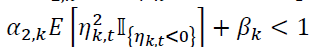
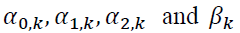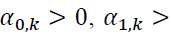
where is the indicator function with a value of 1 if the condition holds and zero otherwise. The GARCH parameters constitute the multi-dimensional vector of the parameter space which is to be estimated. The normal GARCH conditions, 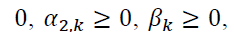are imposed to ensure the variance is strictly positive. We require to guarantee that the returns in each regime is covariancestationary. The choice of the GJR-GARCH was informed by other studies of currency volatility; for example Matei (2009) and Makenzie (2002).

Model Estimation

We estimate the models parameters via either maximum likelihood estimation (MLE) or Markov chain Monte Carlo (MCMC). For both approaches, we evaluate the likelihood given by:

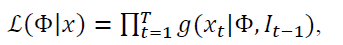
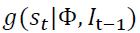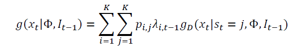
with as the density of given the filtration and the vector of model parameters The regime-switching GARCH conditional density for the returns, is specified as:

where gives the filtered probability of regime i at a time t-1. Billio and Cavicchioli (2017) point out the difficulties in estimating MSGARCH models based on maximum likelihood. Augustyniak (2014) solved this problem by making modifications to the MLE procedure. This we find very problematic. We desire a consistent approach to estimating parameters of regime switching models. We therefore adopt the Bayesian MCMC approach of Bauwens et al. (2010) which was earlier suggested by Das and Yoo (2004). In the Bayesian methodology, our inferences are going to be made on sampling of the posterior generated with the adaptive random-walk Metropolis sampler of Vihola (2012).

Data Analysis

Exploratory Data Analysis

We collected data on the daily ZAR/USD exchange rate for the sample period spanning January 04, 2002 to December 29, 2017, giving us 3998 data points. This period we hope is long enough to uncover any abrupt changes in the trends in the exchange rates. We did a time series plot as shown in Figure 1 to assess the patterns and trends in the exchange rate levels over time.

We can see the continued appreciation of the rand against the dollar from January 2002 to about the fourth quarter of 2003 at slightly below 6 rand to the dollar. From there, it depreciated a little finding itself in the range between 6 and 8 rand to the dollar till the middle of 2008 when it shot up violently remaining volatile until the end of first quarter of 2009 when it recovered pushing strongly against the dollar. This gains against the dollar continued hitting 7 rand to the dollar at the end of the first half of 2011 before embarking on its longest period of depreciation against the dollar at the beginning of the second half of 2011 to its peak period at nearly 17 rand at the beginning of 2016. 2016 and 2017 saw a slightly trending down where the rand recovered somewhat with the rate hovering between 13 and slightly above 14 rand to the dollar at the end of our sample period. The average rate of the exchange rate is 9.0905 rand to the dollar.

We calculated the returns, r_t, by taking the log-differences of the exchange rates. To prevent numerical instability resulting from small numbers, the resulting demeaned returns were converted to percentages before analysis. A plot of these returns in Figure 2 shows the returns on the ZAR/USD have been extremely volatile at times.

Returns of Demeaned ZAR/USD Exchange Rate

A visual inspection of the graph in Figure 2 shows the returns series to be covariancestationary. Volatility clustered are very common in the returns. Comparing Figures 1 and 2, we see a rise in volatility with the depreciation of the rand against the dollar. Volatility was particularly elevated at the end of 2007 to the first quarter of 2008.

We show the distribution of the returns in a histogram on which is imposed a normal curve in Figure 3. The distribution of the returns is nearly symmetrical about zero. Symmetry in the distribution of returns to foreign exchange has been observed by numerous studies that have attributed this phenomenon to interventions by central banks (see for example Perera et al., 2006; Neely, 2001). Another likely reason is the practice of forex traders placing stop-loss orders on trades when volatility exceeds certain limits. Again the distribution shows fat-tails to the right. Cotter and Dowd (2007) studied the phenomenon of fat-tails in forex returns and attributed it to market orders and limit orders. Table 1 presents some descriptive statistics from the returns data series.

Table 1:  Statistics Of The Zar/Usd Return Series
Statistic	Mean	Sd	median	Min	Max	Skew	Kurtosis
Value	0	1.14	-0.06	-7.4	10.55	0.56	4.22

A kurtosis of 4.22 shows the distributions departs from normality. If the returns are normally distributed, we should expect kurtosis to be three. We confirmed this by testing for normality using the Jarque-Bera test which gave us a =3188 with a p-value of nearly zero. To build GARCH models, we need to confirm the presence of GARCH effects in the data. The Engle-LM test with the null hypothesis of no ARCH effects for 12 lags was conducted. The test gave a 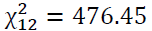and a p-value of almost zero confirming the presence of GARCH effects.

Estimation of MSGARCH Model

We estimated six Bayesian regimes switching GJR (1,1) made of two and three-regimes with both student-t and skewed student-t innovations. We then used the MSGARCH package of Adia et al. (2016) on the R statistical language platform (R Core Team, 2016). The choices are informed by the distribution in Figure 3. We took account of the heavy-tails in the distribution and leverage effects which are normally associated with forex trading (Bredin and Hyde, 2004; Giot & Laurent, 2004). This actually informed our choice of the student-t and skewed student-t errors in modelling. Currency traders routinely employ leverage in trading. This leverage effect is dominant in carrying trades (Acharya and Steffen, 2015).

For the MCMC, we specified 12500 iterations with a burn-in of 5000 and three chains. Some researchers have recommended a burn-in of 4000 (Raftery & Lewis, 1992). Markov chains are not truly independent and identically distributed (Cowles & Carlin, 1996). The idea of thinning Markov chains remains controversial in Bayesian statistics. Some authors, for example, Ruppert (2011); Hadfield (2010); O'Hara and Sillanpää (2009), recommend thinning the posterior draws to reduce the autocorrelations. There is no gold standard for the length of thinning in Bayesian literature (Toft et al., 2007). Others such as Owen (2017) and Geyer (1992) have issues with the usefulness of thinning. Notwithstanding that, we followed the guidelines provided by Spiegelhalter et al. (2003), Brooks et al. (2003) and Gelfand (2000) and chose a thinning length of 10. The graphs of the resulting conditional volatility of our models is as shown in Figure 4.

Model Diagnostics and Fit

We rely on the deviance information criteria (DIC) of Spiegelhalter et al. (2002) as model fit statistics to select the appropriate and parsimonious model from among the lot. Table 2 displays the DIC for each model.

Table 2: Comparison Of Dic Of The Models
Model	DIC
3-regime GJR (1,1) with skewed student-t innovations	16318.92
3-regime GJR (1,1) with student-t innovations	38493.42
2-regime GJR (1,1) with skewed student-t innovations	11707.33
2-regime GJR (1,1) with student-t innovations	11757.19
single-regime GJR (1,1) with skewed student-t innovations	11709.44
single-regime GJR (1,1) with student-t innovations	11749.34

From Table 2, we select the two-regime GJR (1,1) with skewed student-t innovations as the model that best describes the data generation process of the heteroskedastic behaviour. This model provides proof of our suspicion of skewed fat-tails in the distributions of the data. The unconditional volatility of the regimes displayed in Table 3 shows there are clear regimes in the ZAR/USD returns.

Table 3: Unconditional Volatility Of The Models
Model	Regime 1	Regime 2	Regime 3
3-regime GJR(1,1) with skewed student-t innovations	11.6782	20.9959	41.5747
3-regime GJR(1,1) with student-t innovations	12.4399	20.6885	46.6636
2-state GJR(1,1) with skewed student-t innovations	18.6753	31.9956	*
2-state GJR(1,1) with student-t innovations	9.3899	24.635	*
Single-regime GJR(1,1)  with skewed student-t innovations	18.5532	*
Single-regime GJR(1,1) with student-t innovations	18.699	*

The single regime seems to average out the unconditional volatility through some complex averaging scheme. This hides the true evolution of the volatility states of the returns series.

A posterior predictive check of the good-of-fit of our model is necessary in order to draw valid inferences based on the model. We look at the acceptance rate of the MCMC sampler which is 28.4%. This falls within the range of 20%-50% rate recommended by Roberts and Rosenthal (2009). We look at the convergence of the Markov chains by relying on the relative numerical efficiency (RNE) in Table 4. All the values are less than one. This is in line with the recommended values of Geweke (1991).

Table 4: Posterior Estimates Of 2-Regime Gjr(1,1) With Skewed Student-T Innovations
Estimate	Mean	SD	SE	TSSE	RNE
α0,1	0.262	0.2169	0.0069	0.15	0.0021
α1,1	0.0328	0.0301	0.001	0.0108	0.0077
α2,1	0.0001	0	0	0	0.0072
β1	0.6581	0.2167	0.0069	0.0958	0.0051
ν1	49.441	32.0365	1.0131	15.7465	0.0041
η1	0.9489	0.2382	0.0075	0.0703	0.0115
α2,1	0.2307	0.2996	0.0095	0.1323	0.0051
α1,2	0.0674	0.04	0.0013	0.0163	0.006
α2,2	0.0001	0	0	0	0.0093
β2	0.8569	0.059	0.0019	0.01	0.0352
ν2	27.7664	27.6374	0.874	10.9164	0.0064
η2	1.3261	0.2363	0.0075	0.0779	0.0092
ρ11	0.632	0.3575	0.0113	0.2338	0.0023
ρ21	0.2568	0.2684	0.0085	0.1214	0.0049

We calculated the Bayesian credibility intervals for the estimates drawn from the posterior distribution for the 2.5% and 97.5% quantiles. This is shown in Table 5.

Table 5:  95% Credibility Intervals Of Estimates
Estimate				β1	ν1	η1				β2	ν2	η2
2.50%	0.0011	0.0436	0.0001	0.1816	10.2104	0.0218	0.0096	0.0582	0.0001	0.8497	8.2271	0.2884
97.5%	0.1551	0.3776	0.0471	0.9141	72.5427	1.2337	0.0524	0.1409	0.0090	0.9295	44.9396	1.3775

None of the estimates overlap zero. This shows all of them to be significant. The distribution in the tails of regime 1 are heavier than those of regime 2. The 95% posterior intervals for the threshold parameters are distinct and do not span zero. The long run average, differs for each regime. This confirms the existence of two clear regimes. There is also a persistence in the volatility of returns in regime 2 compared to regime one with the persistent GARCH estimate being 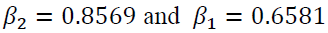respectively.

In all these, the probability of being in regime 1 is 0.1278 which is far less than that of regime 2 which is 0.8722. This shows the dominance of regime 2 which could be due to the volatility of the exchange rate in the last seven years. Low prices for mineral export, one of South Africa's main foreign exchange earner, and political uncertainties in the country have influenced the markets especially the currency market in the latter part of the study period.

Conclusion

Volatility remains topical in finance partly as a result of its latent nature and investors having to estimate it from historical data or infer it from prices of options on assets. Unfortunately, the process of estimating volatility will seem partly an art and partly science (Pierre, 1998). The science part enables us to form a consistent, model-based view of volatility. GARCH models form part of this view. Lamoureux and Lastrapes (1990), however, identified shortfalls of GARCH models including their inability to fully account for persistence in volatility and structural changes. Currencies respond instantly to the changes in the underlying economy and also to the psychology of traders. It is therefore intuitive to model the volatility of foreign exchange returns incorporating regime changes. That is what we achieved in this study.

For currency traders and investors, this research should serve as a key formalization of their knowledge of the behaviour of the volatility of the returns of the Rand/USD exchange rate. We have seen that secular changes on the economy of South Africa push the rand into a dominant high volatility regime. This is a signal for them to adapt their trading strategies and hedge their downside. Mispricing of assets resulting from the under- or over-estimation of risk leads to misallocation of capital. This can result if regimes do not correctly price assets to match market risks (Ammann and Verhofen, 2006). Ichiue and Koyama (2011) opined that markets switching regimes can turn against traders and wipe out their capital.

Policy planners and monetary authorities in South Africa will find this study useful. Tracking the dynamics of the movements in the foreign exchange markets with the regimes could serve as an early warning system of an impending downturn. A depreciating rand induces economic pain across the economy. Depreciation of the rand leads to price inflation of imported goods. This in turn shows up as agitations for increases in wages and upward adjustments in pensions and transfer payments. Extreme currency volatility risks getting out of control and snowballing into other forms of crisis (Chang & Velasco, 2001). For national economies, tensions which accumulate in currency markets reflect some dislocations in the economy, be they trade deficits, the balance of payments issues, fiat legislation against the capital flow or indeed protracted recessions. Monetary and fiscal authorities can study these regime changes and take actions that lean the economy against the winds to lessen the disruptive effects of currency volatility.

References

1. Acharya, V.V., & Steffen, S. (2015). The “greatest” carry trade ever? Understanding eurozone bank risks. Journal of Financial Economics, 115(2), 215-236.
2. Akinboade, O.A., & Makina, D. (2006). Mean reversion and structural breaks in real exchange rates: South African evidence. Applied Financial Economics, 16(4), 347-358.
3. Alexander, P. (2013). Marikana, turning point in South African history. Review of African Political Economy, 40(138), 605-619.
4. Ammann, M., & Verhofen, M. (2006). The effect of market regimes on style allocation. Financial Markets and Portfolio Management, 20(3), 309-337.
5. Augustyniak, M. (2014). Maximum likelihood estimation of the Markov-switching GARCH model. Computational Statistics & Data Analysis, 76, 61-75.
6. Bah, I., & Amusa, H.A. (2003). Real exchange rate volatility and foreign trade: Evidence from South Africa's exports to the United States. African Finance Journal, 5(2), 1-20.
7. Bauwens, L., Preminger, A., & Rombouts, J.V.K (2010). Theory and inference for a Markov switching GARCH model. The Econometrics Journal, 13(2), 218-244.
8. Bhundia, A.J., & Ricci, L.A. (2005). The Rand Crises of 1998 and 2001: What have we learned. Post-apartheid South Africa: The first ten years. 156-173.
9. Billio M., Cavicchioli M. (2017). Markov Switching GARCH Models: Filtering, Approximations and Duality. In: Corazza M., Legros F., Perna C., Sibillo M. (eds) Mathematical and Statistical Methods for Actuarial Sciences and Finance. Springer, Cham.
10. Bollerslev, T. (1986). Generalized autoregressive conditional heteroskedasticity. Journal of Econometrics, 31(3), 307-327.
11. Bredin, D., & Hyde, S. (2004). FOREX Risk: Measurement and evaluation using value?at?risk. Journal of Business Finance & Accounting, 31(9?10), 1389-1417.
12. Brooks, S.P., Giudici, P., & Philippe, A. (2003). Nonparametric convergence assessment for MCMC model selection. Journal of Computational and Graphical Statistics, 12(1), 1-22.
13. Chang, R., & Velasco, A. (2001). A model of financial crises in emerging markets. The Quarterly Journal of Economics, 116(2), 489-517.
14. Cheung, Y.W., & Erlandsson, U.G. (2005). Exchange rates and Markov switching dynamics. Journal of Business & Economic Statistics, 23(3), 314-320.
15. Chiarella, C., He, X.Z., Huang, W., & Zheng, H. (2012). Estimating behavioural heterogeneity under regime switching. Journal of Economic Behavior & Organization, 83(3), 446-460.
16. Cotter, J., & Dowd, K. (2007). The tail risks of FX return distributions: a comparison of the returns associated with limit orders and market orders. Finance Research Letters, 4(3), 146-154.
17. Cowles, M.K., & Carlin, B.P. (1996). Markov chain Monte Carlo convergence diagnostics: a comparative review. Journal of the American Statistical Association, 91(434), 883-904.
18. Das, D., & Yoo, B.H. (2004). A Bayesian MCMC algorithm for Markov switching GARCH models. Econometric Society.
19. De Jong, E., Verschoor, W.F., & Zwinkels, R.C. (2010). Heterogeneity of agents and exchange rate dynamics: Evidence from the EMS. Journal of International Money and Finance, 29 (8), 1652-1669.
20. Dornbusch, R., Goldfajn, I., Valdés, R.O., Edwards, S., & Bruno, M. (1995). Currency crises and collapses. Brookings Papers on Economic Activity. 1995(2), 219-293.
21. Engel, C. (1994). Can the Markov switching model forecast exchange rates? Journal of International Economics, 36(1-2), 151-165.
22. Engle, R.F (2004). Risk and volatility: Econometric models and financial practice. American Economic Review, 94(3), 405-420.
23. Engle, R.F. (1982). Autoregressive conditional heteroscedasticity with estimates of the variance of United Kingdom inflation. Econometrica: Journal of the Econometric Society, 987-1007.
24. Frankel, J. (2007). On the rand: Determinants of the South African exchange rate. South African Journal of Economics, 75(3), 425-441.
25. Gelfand, A.E. (2000). Gibbs sampling. Journal of the American statistical Association, 95(452), 1300-1304.
26. Geweke, J.F. (1991). Evaluating the accuracy of sampling-based approaches to the calculation of posterior moments. Minneapolis, MN, USA: Federal Reserve Bank of Minneapolis, Research Department.
27. Geyer, C.J. (1992). Practical markov chain monte carlo. Statistical Science, 7(4), 473-483.
28. Giot, P., & Laurent, S. (2004). Modelling daily value-at-risk using realized volatility and ARCH type models. Journal of Empirical Finance, 11(3), 379-398.
29. Glick, R., & Rose, A.K. (1999). Contagion and trade: Why are currency crises regional? Journal of international Money and Finance, 18(4), 603-617.
30. Glosten, L.R, Jagannathan, R., & Runkle, D.E. (1993). On the Relation Between the Expected Value and the Volatility of the Nominal Excess Return on Stocks. Journal of Finance, 48(5), 1779-1801.
31. Goutte, S., & Zou, B. (2011). Foreign exchange rates under Markov regime switching model. Center for Research in Economic Analysis, University of Luxembourg.
32. Goutte, S., & Zou, B. (2013). Continuous time regime-switching model applied to foreign exchange rate. Mathematical Finance Letters, 2013.
33. Hadfield, J.D. (2010). MCMC methods for multi-response generalized linear mixed models: the MCMCglmm R package. Journal of Statistical Software, 33(2), 1-22.
34. Huang, W., & Zheng, H. (2012). Financial crises and regime-dependent dynamics. Journal of Economic Behavior & Organization, 82(2-3), 445-461.
35. Huang, W., Zheng, H., & Chia, W.M. (2010). Financial crises and interacting heterogeneous agents. Journal of Economic Dynamics and Control, 34(6), 1105-1122.
36. Huang, W., Zheng, H., & Chia, W.M. (2013). Asymmetric returns, gradual bubbles and sudden crashes. The European Journal of Finance, 19(5), 420-437.
37. Ichiue, H., & Koyama, K. (2011). Regime switches in exchange rate volatility and uncovered interest parity. Journal of International Money and Finance, 30(7), 1436-1450.
38. Kaminsky, G., Lizondo, S., & Reinhart, C.M.C. (1998). Leading indicators of currency crises. Staff Papers, 45(1), 1-48.
39. Kilian, L., & Taylor, M.P. (2003). Why is it so difficult to beat the random walk forecast of exchange rates? Journal of International Economics, 60(1), 85-107.
40. Kumah, F.Y. (2011). A Markov?switching approach to measuring exchange market pressure. International Journal of Finance & Economics, 16(2), 114-130.
41. Lamoureux, C.G., & Lastrapes, W.D. (1990). Persistence in variance, structural change, and the GARCH model. Journal of Business & Economic Statistics, 8(2), 225-234.
42. Lee, H.Y., & Chen, S.L. (2006). Why use Markov-switching models in exchange rate prediction? Economic Modelling, 23(4), 662-668.
43. Matei, M. (2009). Assessing volatility forecasting models: why GARCH models take the lead. Romanian Journal of Economic Forecasting, 4(4), 42-65.
44. McKenzie, M. (2002). The economics of exchange rate volatility asymmetry. International Journal of Finance & Economics, 7(3), 247-260.
45. Neely, C.J. (2001). The Practice of Central Bank Intervention: Looking Under the Hood. Federal Reserve Bank of  St. Louis.
46. O'Hara, R.B., & Sillanpää, M.J. (2009). A review of Bayesian variable selection methods: what, how and which? Bayesian Analysis, 4(1), 85-117.
47. Owen, A.B. (2017). Statistically efficient thinning of a Markov chain sampler. Journal of Computational and Graphical Statistics (forth coming).
48. Panopoulou, E., & Pantelidis, T. (2015). Regime-switching models for exchange rates. The European Journal of Finance, 21(12), 1023-1069.
49. Perera, S., Buckley, W., & Long, H. (2016). Market-reaction-adjusted optimal central bank intervention policy in a forex market with jumps. Annals of Operations Research, 262(1), 1-26.
50. Quarterly Bulletin. (2014, September). South African Reserve Bank.
51. R Core Team. (2016). R: a language and environment for statistical computing. R Foundation for Statistical Computing. Vienna, Austria: https://www.R-project.org/.
52. Raftery, A.E., & Lewis, S.M. (1992). Practical markov chain monte carlo: comment: one long run with diagnostics: Implementation strategies for Markov Chain Monte Carlo. Statistical Science, 7(4), 493-497.
53. Roberts, G.O., & Rosenthal, J.S. (2009). Examples of adaptive MCMC . Journal of Computational and Graphical Statistics, 18(2), 349-367.
54. Ruppert, D. (2011). Bayesian Data Analysis and MCMC. In Statistics and Data Analysis for Financial Engineering. New York, NY: Springer (531-578).
55. Sarantis, N. (1999). Modeling non-linearities in real effective exchange rates. Journal of international money and finance, 18(1), 27-45.
56. Spiegelhalter, D., Thomas, A., Best, N., & Lunn, D. (2003). WinBUGS User Manual. Version 1.4. Cambridge, UK: Medical Research Council Biostatistics Unit.
57. Spiegelhalter, D.J., Best, N.G., Carlin, B.P., & Van Der Linde, A. (2002). Bayesian measures of model complexity and fit. Journal of the Royal Statistical Society: Series B (Statistical Methodology), 64(4), 583-639.
58. St Pierre, E.F. (1998). Estimating EGARCH-M models: Science or art? The Quarterly Review of Economics and Finance, 38(2), 167-180.
59. Toft, N., Innocent, G.T., Gettinby, G., & Reid, S.W.J (2007). Assessing the convergence of markov chain monte carlo methods: An example from evaluation of diagnostic tests in absence of a gold standard. Preventive veterinary medicine, 79(2-4), 244-256.
60. Vihola, M. (2012). Robust adaptive metropolis algorithm with coerced acceptance rate. Statistics and Computing, 22(5), 997-1008.
61. Wilfling, B. (2009). Volatility regime-switching in European exchange rates prior to monetary unification. Journal of International Money and Finance, 28(2), 240-270.
62. Yamamoto, R., & Hirata, H. (2013). Strategy switching in the Japanese stock market. Journal of Economic Dynamics and Control, 37(10), 2010-2022.
63. Yuan, C. (2011). Forecasting exchange rates: The multi-state Markov-switching model with smoothing. International Review of Economics & Finance, 20(2), 342-362.