Keywords

Energy Commodities, Markov Regime-Switching, Crude Oil, Dynamic Relationship.

Introduction

There is considerate literature on energy commodities, their co-movement and causal relationship. The importance of energy commodities also lies in the investor trading which results in prices hikes in financial markets (Baffes & Haniotis, 2010), hedging energy risk with the integration of stock markets (Batten, Kinateder, Szilagyi & Wagner, 2017), linkage with precious metals like Gold, Silver, Palladium, etc., (Bildirici & Turkmen, 2015; Melvin & Sultan, 1990; Sensoy, 2013) and energy-grain nexus (Balcombe & Rapsomanikis, 2008; Sari, Hammoudeh, Chang & McAleer, 2012). In short, it is necessary to understand the underneath dynamics of energy commodities to evaluate energy investment decisions and providing hedging as an alternative to stock and commodity markets.

The previous empirical literature presents evidence for causality between energy commodities. Among the energy commodities, there are numerous studies which suggest the relationship between the crude oil and natural gas. There is mixed evidence for causality which suggests for bidirectional causality (Halova, Wolfe & Rosenman, 2014), a long-run causal relationship (Caporin & Fontini, 2017) and sometimes unstable causality (Batten, Ciner & Lucey, 2017) from the previous researchers. Sari et al. (2012) checked the short run and long-run relationship between the crude oil and gasoline and found that there exists bidirectional relationship in short run which eroded in long run. The correlation between the Crude oil, Gasoline, heating oil, kerosene, propane, etc., is checked and evident for their positive relationship (Block, Righi, Schlender & Coronel, 2015).

This study adds a new dimension, contribute and fill in the existing literature through two different perspectives. First, historical events affect the time-series severely, but the single mean and standard deviation are used in the previous empirical literature (Batten, Ciner & Lucey, 2017; Block et al., 2015; Caporin & Fontini, 2017). We used Markov regime-switching model (MRSM) which take separate means and standard deviation for each regime and hence, remove any kind of misspecification in modelling arise. Secondly, the most important methodological improvement is to compute regimes automatically through the algorithm design of MRSM which can generate two models for forecasting rather than use a holistic model which governs predictable forces to forecast (Hamilton, 1994). Block et al. (2015) used Copula-DCC-GARCH method to detect a structural break in the correlation series between energy commodities but could not show the magnitude of each regime clearly and their persistence. The structural breaks are inserted to identify the relation between oil and gas through vector error corrected model (Caporin & Fontini, 2017); commodity boom as to check the co-movement in between crude oil and commodity markets (Lucotte, 2016); several structural break in commodity markets (de Nicola, De Pace & Hernandez, 2016); and the sub-periods as structural breaks in US Bio-fuel industry (Gardebroek & Hernandez, 2013). The predictable forces and contemporaneous relationships between prices of energy commodities are deduced through Markov switching model which provide leverage of many regimes.

The paper is organized as follows. Section 2 describes data followed by the estimated methodology in Section 3. Section 4 discusses empirical results. Section 5 concludes.

Data

This paper used the time-series data on the closing spot prices of four widely traded energy commodities which includes the Crude oil, Gasoline, Diesel and Aviation Turbine fuel (ATF). Specifically, the data represents West Texas Intermediate (WTI) spot prices (Dollar per Barrel), New York Harbor Conventional Gasoline Regular Spot Price (Dollars per Gallon), Ultra-Low Sulfur CARB Diesel Spot Price- Los Angeles, CA (Dollars per Gallon) and US Gulf Coast Kerosene-Type Jet Fuel Spot Price (Dollars per Gallon) as Crude oil, Gasoline, Diesel and ATF, respectively. The data is extracted from the US Energy Information Administration website. Descriptive statistics for the four time-series are mentioned in Table 1. The four time-series are used after considering their first difference. The Augmented Dickey-Fuller test (ADF) and Phillip-Perron (PP) test suggest that the data is stationary or not contains the unit-root. For the visual assessment, Figure 1 depicts the time-series of four variables for both original series and first difference of time-series. Jaque-Bera test (JB) is the joint hypothesis to test the skewness and excess kurtosis being zero for which we reject the null hypothesis. The serial correlation is present in the time-series suggested by Ljunx-Box (LB Q-stat) test.

Table 1: Descriptive Statistics
	Crude Oil	Gasoline	Diesel	ATF
Mean	0.1375	0.0046	0.0043	0.0047
Standard Deviation	5.0657	0.1583	0.1586	0.1558
Skewness	-1.2056	-1.1143	-0.8195	-1.9976
Kurtosis	4.6237	4.2973	2.9006	10.3905
Jaque-Bera	298.99	257.83	122.56	1357.6
ADF	-8.179	-10.918	-9.576	-8.655
PP	-10.671	-11.579	-11.936	-13.054
LB Q-stat	38.043 (0.0000)	21.636 (0.0000)	19.761 (0.0000)	11.229 (0.0008)

 Estimated Methodology

In order to build the MRSM model, the first step is to select the optimal lag length according to Schwarz Information Criteria (SIC) which allows the minimum information loss when approximating to the reality (Kullback & Leibler, 1951) and does better for large sample size (Lütkepohl, 1999). Using the 1 lag obtained from the SIC, we conducted the Granger causality test to compare the two models. The one model comprises the past values of both independent variable and dependent variables, which is regressed to the present value of dependent variable. The other model contains only the dependent variable which is regressed to its own past values. By comparing the residual sum of squared errors, F-statistics is used to determine which model works better (Granger, 1969).

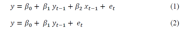
Where y denote the dependent variable, x denotes the independent variable and e is the error term. Till now, the test is for only one variable and only in one direction. We modelled the Granger causality test to operate for bidirectional and for four variables.

Consider an MRSM model where the relationship of Crude oil is established with other energy commodities due to the direction of causality from Crude oil to other energy commodities (Table 2). Let O and E represents the returns series of Crude oil (independent variable) and other energy commodities (Gasoline, Diesel, ATF as dependent variables), respectively. In the two-state Markov regime-switching model of order q (MS-AR(k)):

Table 2: Granger Causality Test
Granger Causality	F-Statistic (1 lag)	P-value
Crude oil prices granger cause Gasoline prices Gasoline prices does not granger cause Crude oil prices	6.0744 0.0416	0.0144** 0.8386
Crude oil prices granger cause Diesel prices Diesel prices does not granger cause Crude oil prices	9.1251 0.3019	0.0027*** 0.5832
Crude oil prices granger cause Aviation Turbine fuel prices Aviation Turbine fuel prices does not granger cause Crude oil prices	19.748 0.1758	0.0000*** 0.675

Note: Table 2 describes the direction of causality of energy commodities for 1 lag length. The correspond p-values suggest whether variable granger cause to other variables. ***, ** and * significant at level 1%, 5% and 10%, respectively.

Where and are the state-dependent mean and variance, respectively. The state-dependent coefficients 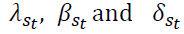represent the lagged relation and contemporaneous relationship of Crude oil with energy commodities and autocorrelation of other energy commodities, respectively. The switching between the regimes, s_t, takes the values of either 1 or 0 depends in which regime the variable is in. The two-state markov process is followed by both dependent and independent variables with a fixed transition probability matrix:

Empirical Results

The contemporaneous and causal relationship between energy commodities is tested through Markov regime-switching process of AR (0) and AR (1), respectively. The lag length, 1 lag, is determined for this purpose according to SIC criteria. Further, the Granger causality test is performed in order to know the direction of causality for energy commodities. The results in Table 2 show that the crude oil granger causes the Gasoline, Diesel and Aviation turbine fuel (ATF) but not vice-versa. Thus, we applied the two-state MRSM by considering only 1 lag length to test the contemporaneous and dynamic relationship of crude oil with other energy commodities according to Equation (3).

The likelihood function of the model with regime-switching has the higher value than does the ordinary linear model (without regime-switching or one regime model). The Likelihood ratio (LR) statistic is 76.2, 36.54 and 151.54 for the relationship of Crude oil with Gasoline, Diesel and ATF, respectively. Due to nuisance parameter problem in comparison, Garcia (1998) provided critical values for MRSM model which is 14.02 at 99% confidence interval. This value is less than the LR statistic suggests that MRSM model outperforms the ordinary linear model.

Previous empirical literature is silent about the precise definition of bull and bear market (Candelon, Piplack & Straetmans, 2008). The state with high mean-low variance can be defined as bull (upward) market state and the state with low mean-high variance can be defined as bear (downward) market state. Crude oil-Diesel has the mixed signal of mean and variance; we decided to go with variance as the difference between the two means is not significant. We can clearly define the upward and downward market state according to mean and variance, for example, μ₀ and σ₀ relate to the upward market state and μ₁ and σ₁ relate to downward market states.

Table 3: Markov Regime-Switching Estimation
	(1)		(2)		(3)
	MS-AR(0)	MS-AR(1)	MS-AR(0)	MS-AR(1)	MS-AR(0)	MS-AR(1)
μ0	0.0015 (0.004)	0.0013 (0.004)	0.0003 (0.0037)	-0.0014 (0.0047)	0.0028 (0.0032)	0.0021 (0.0023)
μ1	0.0009 (0.0119)	0.0007 (0.0089)	0.0018 (0.0087)	0.0026 (0.0088)	-0.0027 (0.0164)	-0.0003 (0.0668)
σ0	0.0406	0.0405	0.0467	0.0455	0.0396	0.0349
σ0	0.1184	0.1185	0.1065	0.106	0.1461	0.1309
β0	0.0263*** (0.0015)	0.0264*** (0.0015)	0.0256*** (0.0018)	0.025*** (0.0017)	0.0251*** (0.0011)	0.0259*** (0.0014)
β1	0.0249*** (0.0017)	0.0251*** (0.0018)	0.0269*** (0.0016)	0.0269*** (0.0016)	0.0267*** (0.0025)	0.0253*** (0.0022)
λ0	-	0.0011 (0.003)	-	0.0069* (0.0029)	-	0.0055* (0.0023)
λ1	-	-0.0015 (0.0028)	-	0.0001 (0.002)	-	0.0034 (0.0028)
δ0	0.019 (0.0511)	-0.0482 (0.0986)	0.1078* (0.0633)	-0.0771 (0.1014)	0.0125 (0.0317)	-0.1876* (0.0868)
δ1	0.044 (0.0556)	0.0796 (0.0865)	-0.0384 (0.0515)	-0.0403 (0.0688)	-0.0871 (0.08)	-0.1403 (0.0958)
p00	0.957	0.956	0.952	0.957	0.963	0.968
p11	0.956	0.954	0.957	0.961	0.904	0.94
Log-Lik	290.2	290.39	284.3	287.09	339.8	342.36

Note: Estimates and standard error in brackets are given. MS-AR(0) and MS-AR(1) processes have state-dependent mean (μ0, μ1) and variances () in each regime. (1), (2) and (3) signifies the relationship of Crude oil with Gasoline, Diesel and, ATF, respectively. ***, ** and * significance at the 0.1%, 1% and 5% level, respectively.

The results of MRSM estimation in Table 3 show that all β₀ and β₁ are more than zero which suggests that Crude oil is contemporaneously and positively related to the Gasoline, Diesel and ATF in both upward and downward market state. The results are robust for MS-AR(0) and MS-AR(1) process. With the one lag included in the model allows us to test for dynamic or causal relationship of crude oil with other energy commodities. Not as the same of contemporaneous relationship, Crude oil has causal affect only on Diesel and ATF but not on Gasoline. With the analysis of monthly prices, it is obvious to have less than or equal to one month causal effect because market demand and supply forces brings back their prices in equilibrium. The force happened only in upward market state which suggests the possibility of trend following as an old proverb of Wall Street says “In a bull market, be bullish”. In nutshell, the crude oil has predictive power (positive) over Diesel and ATF in upward market state only. Surprisingly, the autocorrelation of energy commodities (Diesel and ATF) happened only in upward market state where the Diesel has positive relation with its past value while ATF has negative relation with ATF_t-1.Table 4 reports the persistence period for both regimes for both AR processes. These persistence periods are calculated from the transition probabilities. The upward market state persists for around 23 months and around 21-23 months; and the downward market state persists for around 22-23 months and 23-26 months for Crude oil to Gasoline and Diesel relation, respectively. Surprisingly, the Crude oil and ATF relation exhibit asymmetric relationship in bull and bear market. The upward market state holds for around 27-31 months while the downward market state exists for around 10-17 months. This exhibits the tendency to move together in the upward market state but weak tendency to move together in the downward market state. The demand forces and upward market trend of Crude oil lead the prices of ATF in upward direction. As ATF is used in the aviation sector for which the utility is a lot different from Crude oil, the supply forces cannot govern the prices of ATF to move into downward direction. Thus, this may be the reason due to which the asymmetric effect arises between both market states.

Table 4 : Persistence Period For Each Regime
	Upward (1)	Downward (1)	Upward (2)	Downward (2)	Upward (3)	Downward (3)
MS-AR(0)	23.26	22.73	20.83	23.26	27.03	10.42
MS-AR(1)	22.73	21.74	23.26	25.64	31.25	16.67

Note: (1), (2) and (3) represents the results for crude oil-gasoline, crude oil-diesel, crude oil-ATF, respectively. Regimes 1 and 2 represent upward and downward market states, respectively. All values are in months.

Figure 2 depicts the same persistence phenomena through the smoothed and filtered probabilities in Regime 1 (upward market state) on the relationship between Crude oil with energy commodities. This method is also adopted to demonstrate the hidden structural breaks and historical events over the time in the form of ups and downs in the graph. The downs starting from mid-2004 till the October 2008 are the reflection of the events such as Venezuelan strike and Iraq war (2003-2004), Hurricanes (2004-2005), Ethanol used as a replacement of MTBE (methyl t-butyl ether) (2006) and Oil price spike (2007-2008); while the reflection of the events happened between the year 2009 to year 2015 depicted as the downs. The events happened during this tenure are mainly the stock market shocks which impacted at commodity markets such as e.g. Global recession (2008), Liquidity and credit crunch (2007-2008), Sub-prime crisis (2007-2009), the automotive industry crisis (2008-2010), Arab uprising and Unrest in Libya (2010-2011), Excess capacity (supply) (2014-2015) and Crash in Crude oil prices due to Overproduction in US and Russia (2014-2015), etc. Thus, the MRSM provide us with the automatic predictive tool to forecast the future and investigate the past.

Concluding Remarks

This paper examines the relationship of Crude oil with other energy commodities through the MRSM. We report the evidence that there exists a contemporaneous relationship between the Crude oil with Gasoline, Diesel and ATF and causal relationship effect is detected between Crude oil with Diesel & ATF only in the upward market state. The evidence suggests that trend following strategy govern the mechanism between the Crude oil with Diesel and ATF. The upward and downward market states are highly persistent in each case. The asymmetric effect for Crude oil-ATF suggests the weak tendency to move together in the downward market state. This may be due to the special utility of ATF in aviation sector which is a way different with the utility of Crude oil. Thus, the rules or forces governing the Crude oil-ATF in bull market weakly govern the relationship in a bear market. Our study also demonstrates the structural breaks happened in the past through the ups and downs in the smoothed and filtered probabilities which is a very interesting aspect of this study. The study will be useful for the global investors in commodity, especially in energy commodities to align their trading strategy with the market patterns and co-movement behavior of energy commodities in bull and bear markets.

Acknowledgment

This research is supported by a research grant from Indian Institute of Management Raipur.

References

1. Baffes, J. & Haniotis, T. (2010). Placing the 2006/2008 commodity price boom into perspective. World Bank Development Prospects Group (Vol. Policy Res).
2. Balcombe, K. & Rapsomanikis, G. (2008). Bayesian estimation and selection of nonlinear vector error correction models: The case of the sugar-ethanol-oil nexus in Brazil. American Journal of Agricultural Economics, 90(3), 658-668.
3. Batten, J.A., Ciner, C. & Lucey, B.M. (2017). The dynamic linkages between crude oil and natural gas markets. Energy Economics, 62, 155-170.
4. Batten, J.A., Kinateder, H., Szilagyi, P.G. & Wagner, N.F. (2017). Can stock market investors hedge energy risk? Evidence from Asia. Energy Economics, 66, 559-570.
5. Bildirici, M.E. & Turkmen, C. (2015). Nonlinear causality between oil and precious metals. Resources Policy, 46, 202-211.
6. Block, A.S., Righi, M.B., Schlender, S.G. & Coronel, D.A. (2015). Investigating dynamic conditional correlation between crude oil and fuels in non-linear framework: The financial and economic role of structural breaks. Energy Economics, 49, 23-32.
7. Candelon, B., Piplack, J. & Straetmans, S. (2008). On measuring synchronization of bulls and bears: The case of East Asia. Journal of Banking and Finance, 32(6), 1022-1035.
8. Caporin, M. & Fontini, F. (2017). The long-run oil–natural gas price relationship and the shale gas revolution. Energy Economics, 64, 511-519.
9. de Nicola, F., De Pace, P. & Hernandez, M.A. (2016). Co-movement of major energy, agricultural and food commodity price returns: A time-series assessment. Energy Economics, 57, 28-41.
10. Garcia, R. (1998). Asymptotic null distribution of the likelihood ratio test in markov switching models. International Economic Review, 39(3), 763-788.
11. Gardebroek, C. & Hernandez, M.A. (2013). Do energy prices stimulate food price volatility? Examining volatility transmission between US oil, ethanol and corn markets. Energy Economics, 40, 119-129.
12. Granger, C.W.J. (1969). Investigating causal relations by econometric models and cross-spectral methods. Econometrica, 37(3), 424.
13. Halova, W.M. & Rosenman, R. (2014). Bidirectional causality in oil and gas markets. Energy Economics, 42, 325-331. https://doi.org/10.1016/j.eneco.2013.12.010
14. Hamilton, J.D. (1994). Time Series Analysis. Princeton University Press, New Jersey.
15. Kullback, S. & Leibler, R.A. (1951). On information and sufficiency. The Annals of Mathematical Statistics. Institute of Mathematical Statistics.
16. Lucotte, Y. (2016). Co-movements between crude oil and food prices: A post-commodity boom perspective. Economics Letters, 147, 142-147.
17. Lütkepohl, H. (1999). Vector autoregressions. Interdisciplinary Research Project (Discussion Paper), 4.
18. Melvin, M. & Sultan, J. (1990). South African political unrest, oil prices and the time varying risk premium in the gold futures market. Journal of Futures Markets, 10(2), 103-111.
19. Sari, R., Hammoudeh, S., Chang, C.L. & McAleer, M. (2012). Causality between market liquidity and depth for energy and grains. Energy Economics, 34(5), 1683-1692.
20. Sensoy, A. (2013). Dynamic relationship between precious metals. Resources Policy, 38(4), 504-511.