Research Article: 2020 Vol: 24 Issue: 2
Return and Volatility Spillovers Between Stock and Futures Markets in Thailand
Purichita Sukhonpitumart, RHB Securities
Anutchanat Jaroenjitrkam, Thammasat University
Sakkakom Maneenop, Thammasat University
Chaiyuth Padungsaksawasdi, Thammasat University
Abstract
We examine return and volatility spillovers between the SET50 index futures and its underlying index in the Thai financial exchanges. The findings show that the return of the spot market leads that of the futures market. Of three bivariate GARCH families, the GJR-GARCH model best describes the volatility movement. Moreover, bad news is more influential on the volatility spillover than good news, documenting an asymmetric effect. There exists a bidirectional volatility spillover, but the spillover from the futures market to the spot market is more notable during the recent sub-periods.
Keywords
Spillover, Return, Volatility, SET50 index, GARCH, EGARCH, GJR-GARCH.
JEL Classifications
G12, G13
Introduction
There are voluminous studies on spillover effects between spot and its associated futures markets in various financial instruments, for example, equities (Tse, 1995), bonds (Skintzi & Refenes, 2006), exchange rates (Chatrath & Song, 1998), and commodities (Liu, Cheng, Wang, Hong & Li, 2008). Prior literature in equity markets shows different findings between developing and developed markets. Spillovers from futures markets to their spot markets are usually found in developed markets; however, the results seem to be mixed in developing markets. This paper provides additional evidence in this regard. We examine the return spillover and volatility spillover between the stock market return (SET50) and its corresponding stock index futures because derivative markets in Thailand are still young, and lack empirical evidence. The SET50 index futures as the first derivative product in the exchange was launched in April 2006 and have gained popularity since then. Moreover, investors in the Stock Exchange of Thailand comprise local institutions, proprietary, foreign, and retail (individual) traders, of which a majority is retail traders usually considered as uninformed traders. Lertweeranontharat et al. (2016) conclude that noise trader is the major player in the Thailand Futures Exchange, measuring by the higher ratio between uninformed traders and informed traders in Thai than that in developed markets. These unique characteristics are different from developed markets, which gives us an opportunity to investigate the investors’ behavior of information transmissions between these two markets. This potentially differs from prior evidence in developed markets. To investigate spillovers between the spot and futures markets, we first examine the lead-lag relationship in stock index returns and stock index volatility both in spot and futures markets. Judge & Reancharoen (2014) emphasize the lead-lag relationship between the SET50 index and its associated futures in Thailand. Our study differs from them by employing several GARCH models over a long sample period. Generally, the results are consistent with their findings. Second, we determine which econometric model is the best fit in explaining the spillover effects in the Thai financial markets. Last, we in-depth analyze subsample periods determined by Bai & Perron’s (1998) methodology in order to explore structural shifts in the spillover effect.
Our results show that the GJR-GARCH model is the most effective model in explaining the long memory behavior of volatility in the Thai financial markets. Unlike the findings in developed markets (Abhyankar, 1995; Tse, 1999), we find that the returns of the spot market lead those of its associated futures market. An information transmission between spot and futures markets is observed with a greater effect from the spot market to the futures market. In addition, the volatility spillover from the futures market to the spot market becomes more significant during the recent periods.
Review of Literature
Evidence in international developed financial markets shows that information spills from the futures market to its associated spot market. Abhyankar (1995) finds that the FTSE-100 futures market leads the spot market at hourly interval data. Iihara et al. (1996), employing intraday data in Japanese market, find the volatility spillover from the futures market to its associated stock market. This is consistent to the findings of Bhar (2001) in Australia & Lafuente (2002) in Spain. Tse (1999) finds a bidirectional volatility spillover in the U.S. markets and the impact from the futures market to the spot market is stronger. However, evidence in emerging markets is mixed. Lin et al. (2002) demonstrate the bidirectional Granger causality and strong volatility spillover from the stock to the futures markets. Zhong et al. (2004) find that the return of the futures market leads that of the spot market in Mexico, but the evidence is opposite for volatility spillover. Ba?da? (2009) finds that the Istanbul Stock Exchange 30 index return leads its futures return, and Streche (2009) finds the similar results in Romania. However, Pati & Rajib (2011) indicate the unidirectional return spillover from the futures to the spot markets in the Indian exchange. Finally, Jin & Yang (2013) find a unidirectional volatility spillover from the Chinese CSI spot market to the futures market.
An important aspect of the spillover effect is an asymmetric effect. Booth, Martikainen, & Tse (1995), employing EGARCH in Scandinavian countries, indicate that bad news has more impact on spillover effect than good news. The conclusion is also confirmed by Bhar (2001) in Australia & Lin (2002) in Taiwan. However, Kang & Yoon (2013), employing GJR-GARCH to investigate the return and volatility linkages in foreign exchange and stock markets in Korea, do not find an asymmetric effect. Moreover, previous studies report a decline in spillover or a shift in estimated parameters, implying potential structural breaks, for example an increase in the margin level in futures market (Iihara et al., 1996) and a decrease in the size of futures contract (Bhar, 2001). Therefore, we include an effect of structural breaks in this study.
Data
Daily prices of the SET50 index futures and those of the SET50 index1 are from DataStream. The daily average volume of the SET50 index futures is 300,000 contracts over the examined period. Different maturity contracts are available, including three nearest consecutive months and end of the March, June, September, and December.
The study period starts from January 3, 2007 to April 29, 2014. The data in year 2006, which is the established year, are excluded due to illiquidity at the early stage of the market. According to the Samuelson (1965) effect2 presented in the SET50 index futures suggested by Dolsutham et al. (2011) and Lertweeranontharat et al. (2016), time series data are created by using prices of the nearest quarterly month contract, which is the closest maturity at the end of each quarter.
Methods and Methodology
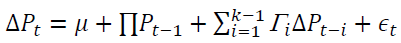
We start our analyses to validate the stationary property of the variables by using the Augmented Dickey-Fuller (1979) test. The two-period optimal lag length is determined by the Akaike Information Criterion (AIC). Next, the futures-stock index relationship using Johansen (1988) cointegration is investigated as
 (1)
(1)
where 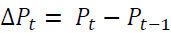 and
and vector of log of prices in spot and futures markets at time
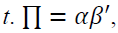 which
which vectors, and r is a cointegrating rank of the system.
Conditional Mean
The return spillover between spot and futures markets is examined by using a lead-lag relationship. We include an error correction term in a bivariate equation as cointegration exists between these two markets as shown below.
 (2)
(2)
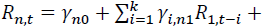
 vector of the rate of return of asset n at time t, where n equals 1 and 2 for spot and futures markets, respectively. k is the AIC optimal lag length.
 is an error correction term of asset n, which is the lag of residual obtained from Equation (1).
 shows the return spillover from futures market to spot market, and describes the return spillover from spot market to futures market.
 denotes lag operations.
Conditional Variance
The study explores the volatility spillover between spot and futures markets by employing three GARCH models that are GARCH, EGARCH, and GJR-GARCH.
GARCH Model
A bivariate GARCH is shown below.
 (3)
(3)

where 1 and 2 represent the SET50 index and the SET50 index futures, respectively.  is the conditional variance of asset n at time
 explains persistence in volatility at lag j of asset
 is the i-th lag of a white noise of asset n.
 capture the impact of the i-th lag of standardized innovations of the same market, while
 describe the impact of cross-market standardized innovations between the spot and futures markets.
GARCH model treats symmetrically an effect of positive and negative information. However, several studies show that markets respond to bad and good news differently (Veronesi, 1999 and Giner and Rees, 2001). We further study by employing EGARCH model (Nelson 1991), and GJR-GARCH model (Glosten, Jagannathan, and Runkel 1993).
EGARCH Model
A bivariate exponential GARCH (EGARCH) model is shown below.
 (4)
(4)


 allow an asymmetric effect in the model.
 and
and capture the size effect implying if the absolute value is greater than its expected value, the volatility will increase.
 identify the sign effect. When
  and Z are negative, the volatility will increase higher than when Z is positive.
 is the parameter measuring persistence in volatility at lag j of asset
 capture the impact of the i-th lag of innovations of the same market, while
 explain the impact of cross-market standardized innovations between spot and futures markets.
GJR-GARCH model
A bivariate GJR-GARCH model is designed to capture an increased volatility from asymmetric shocks, which is also known as the leverage effect, presented as follows.
 (5)
(5)
where 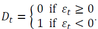 The GJR-GARCH implies when
 negativity amplifies the conditional variance.
 is the conditional variance.
 measures persistence in volatility.
 is the i-th lag of a white noise. The impact of the white noise on the conditional variance is measured by
  when
when  and by
The maximum likelihood is used to estimate the variables in all models mentioned previously. Finally, we want to find which model works best in our setting. The root mean squared error (RMSE) as a measure of model efficacy is used for the three GARCH models. The model with the smallest RMSE, which is the best fit model, is the baseline model for a further study in structural break analysis. The measurement of RMSE is demonstrated in Equation (6).
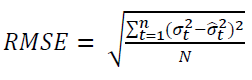 (6)
(6)
where  is the realized volatility at time
 is the estimated volatility from GARCH, EGARCH, and GJR-GARCH.
Empirical Results
Table 1 presents the descriptive statistics of the stock index return and its futures return with the normality test. In general, the return on stock and its corresponding futures markets are indifferent with a slightly higher variance in the futures market. Jarque Bera statistics show the nonnormality of the both variables.
| Table 1 Descriptive Statistics of Return of Set 50 Index and Set 50 Index Futures | ||||||
| Mean (*10-4) | Variance | Skewness | Kurtosis | Jarque Bera | ADF | |
| SET50 index | 4.12 | 2.53 | -0.4853 | 6.1639 | 62.9826*** | -1721.48*** |
| SET50 index futures | 4.11 | 3.41 | -0.2686 | 5.6074 | 60.4895*** | -1890.78*** |
Table 2 presents the results of the cointegration test. We cannot reject the null hypothesis of rank ≤ 1, but reject the null hypothesis of rank = 0, showing that there exists at least one cointegrating rank in the system. In conclusion, the spot prices and futures prices demonstrate a long-run relationship in the equilibrium condition.
| Table 2 Cointegration Test for the Spot and Futures Markets | ||
| H0: Rank = r | Trace Statistic | 5% Critical Value |
| 0 | 127.0333 | 12.21 |
| 1 | 0.9363 | 4.14 |
Conditional Mean
Table 3 demonstrates the estimation of conditional mean obtained from a bivariate VAR model with the four AIC optimal lag lengths.  demonstrate a unidirectional return spillover from the spot market to the futures market. However,
 are insignificant, showing no return spillover effect from the futures market to spot market. The evidence is consistent with the finding of Basdas (2009) in Turkey.
7
| Table 3 The stock-futures return spillover | |||
| Spot | Futures | ||
| Parameter | Coefficient | Parameter | γCoefficient |
| γ10 | 0.043 | γ20 | 0.0418 |
| (1.14) | (0.97) | ||
| γ1,11 | 0.2484 | γ1,21 | 0.4619* |
| (1.20) | (1.93) | ||
| γ1,12 | -0.1665 | γ1,22 | -0.4159** |
| (-0.95) | (-2.05) | ||
| γ2,11 | 0.1002 | γ2.21 | 0.3054** |
| (0.90) | (2.38) | ||
| γ2,12 | -0.0602 | γ2,22 | -0.2634** |
| (-0.57) | (-2.18) | ||
| γ 3,11 | -0.1326 | γ3,21 | 0.0442 |
| (-1.43) | (0.41) | ||
| γ 3,12 | 0.1046 | γ3,22 | -0.0877 |
| (1.25) | (-0.91) | ||
| γ 4,11 | 0.0829 | γ4,21 | 0.1533 |
| (0.99) | (1.59) | ||
| γ 4,12 | -0.0931 | γ4,22 | -0.1532 |
| (-1.25) | (-1.77) | ||
| δ1 | 0.01938 | δ2 | 0.03104 |
| (0.60) | (0.72) | ||
 where
where is the return of asset n at time t. n = 1 and 2 stand for the spot and futures markets, respectively. k is the AIC optimal lag length. Numbers in parentheses indicate t-statistics. *, **, *** denote the statistical significance at 10%, 5%, and 1% levels, respectively.
Conditional Variance
Appropriate models with the AIC optimal lag length are GARCH (1,1), EGARCH (2,2), and GJR-GARCH (3,3). The results in Table 4 exhibit the estimation of GARCH as shown in Equation (3).  showing persistence of volatility in both markets, are statistically significant. A statistical significance of
 reveals the impact of its own market lagged standardized innovations. However,
 are not significant, meaning that there exists no impact from the cross market standardized innovations between the spot and futures markets. Our evidence contradicts to the findings in prior literature. For example, Lin et al. (2002) find the bidirectional volatility spillover between spot and futures markets in Taiwan, while Jin and Yang (2013) discover the unidirectional volatility spillover from spot market to futures market in China.
| Table 4 The Stock-Futures Volatility Spillover of Garch (1,1) Model | |||
| Spot | Futures | ||
| Parameter | Coefficient | Parameter | Coefficient |
| ω1 | 0.0288*** | ω2 | 0.0266*** |
| (2.89) | (2.64) | ||
| α1,11 | 0.1677*** | α1,21 | 0.0404 |
| (3.04) | (0.87) | ||
| α1,12 | -0.0417 | α1,22 | 0.0705* |
| (-0.87) | (1.75) | ||
| β1,1 | 0.8721*** | β1,2 | 0.8927** |
| (58.37) | (75.34) | ||
The table shows the estimated coefficients from the variance equation of 
 where
where is the conditional variance of asset n at time t. n = 1 and 2 stand for the spot and futures markets, respectively. p and q are the AIC optimal lag lengths. Numbers in parentheses indicate t-statistics. *, **, *** denote the statistical significance at 10%, 5%, and 1% levels, respectively.
Table 5 demonstrates the estimation of EGARCH. A statistical significance of 
 presents the bidirectional volatility spillover between the spot and the futures markets both lags. It is interesting to note that a negative spillover from the spot market to the futures market exists during the period t-1.
| Table 5 The Stock-Futures Volatility Spillover of Egarch (2,2) Model | |||
| Spot | Futures | ||
| Parameter | Coefficient | Parameter | Coefficient |
| ω1 | -0.1267*** | ω2 | -0.0973*** |
| (-5.01) | (-3.94) | ||
| α1,11 | 0.0275** | α1,21 | -0.0426*** |
| (2.28) | (-4.54) | ||
| α1,12 | 0.058*** | α1,22 | -0.0475*** |
| (4.75) | (-5.78) | ||
| α2,11 | 0.1312*** | α2,21 | 0.0535** |
| (3.00) | (2.53) | ||
| α2,12 | 0.079** | α2,22 | 0.046*** |
| (2.50) | (2.58) | ||
| β1,1 | 0.7934*** | β1,2 | 0.5921*** |
| (5.53) | (4.15) | ||
| β1,2 | 0.1805 | β2,2 | 0.3871*** |
| (1.28) | (2.74) | ||
| θ1,1 | 6.1334*** | θ1,2 | 8.7813*** |
| (7.62) | (9.66) | ||
| θ1,2 | 3.1026*** | θ2,2 | -7.4025** |
| (2.77) | (-2.31) | ||
The table shows the estimated coefficients from the variance equation of  where
where is the conditional variance of asset n at time t. n = 1 and 2 stand for the spot and futures markets, respectively. p and q are the AIC optimal lag lengths. Moreover,
 and
and
 Numbers in parentheses indicate t-statistics. *, **, *** denote the statistical significance at 10%, 5%, and 1% levels, respectively.
The results of EGARCH estimation are superior to those of GARCH estimation, implying that asymmetric spillover effect appears in the Thai markets. EGARCH model captures an asymmetric effect with the statistical significance of The positive signs of
 imply that good news potentially amplifies an effect on volatility spillover more than bad news, which is different from the finding of previous literature on negative signs of
  for example, Booth et al. (1997) in Scandinavia, Bhar (2001) in Australia, and Lin et al. (2002) in Taiwan.
The estimation of GJR-GARCH is presented in Table 6.  are statistically significant. This implies that bad news is more influential on volatility than good new. However, the results whether bad news increases or decreases volatility are mixed due to the mixed signs of . We can only infer that the most recent bad news raises the volatility from the positive sign of lagged one of
 Moreover, the GJR-GARCH model shows the bidirectional volatility spillover between two markets as
 significant. It is interesting to note that only
 shows a positive spillover, while the others do oppositely. However, the absolute value of is greater than that of
 we can infer that the volatility spillover from the spot market to the futures market is greater than the effect of the reverse direction. Moreover, most lagged variances
 are statistically significant, showing a long memory of volatility.
| Table 6 The Stock-Futures Volatility Spillover Of Gjr-Garch (3,3) Model | |||
| Spot | Futures | ||
| Parameter | Coefficient | Parameter | Coefficient |
| ω1 | 0.0011*** | ω2 | 0.0845*** |
| (6.12) | (3.55) | ||
| α1,11 | 0.0053*** | α1,21 | -0.2226*** |
| (40.66) | (-7.17) | ||
| α1,12 | 0.0332*** | α1,22 | 0.1476*** |
| (26.35) | (5.95) | ||
| α2,11 | 0.0735*** | α2,21 | 0.1057 |
| (55.95) | (1.19) | ||
| α2,12 | -0.0697*** | α2,22 | -0.0046 |
| (-67.6) | (-0.06) | ||
| α3,11 | -0.0910*** | α3,21 | 0.0181 |
| (-141.21) | (0.43) | ||
| α3,12 | 0.0467*** | α3,22 | 0.0624 |
| (41.77) | (1.56) | ||
| β1,1 | 0.9380*** | β1,2 | 0.2996*** |
| (588.78) | (5.90) | ||
| β2,1 | 0.8255*** | β2,2 | 0.0492 |
| (328.88) | (1.08) | ||
| β3,1 | -0.7641*** | β3,2 | 0.4067*** |
| (-446.87) | (9.36) | ||
| τ1,1 | 0.1556*** | τ1,2 | 0.1690*** |
| (66.56) | (4.61) | ||
| τ2,1 | -0.0344*** | τ2,2 | 0.1397*** |
| (-92.09) | (2.68) | ||
| τ3,1 | -0.1194*** | τ3,2 | -0.1019*** |
| (-50.65) | (-3.74) | ||
The table shows the estimated coefficients from the variance equation of 
 where
where is the conditional variance of asset n at time t. n = 1 and 2 stand for the spot and futures markets, respectively. p and q are the AIC optimal lag lengths. Numbers in parentheses indicate t-statistics. *, **, *** denote the statistical significance at 10%, 5%, and 1% levels, respectively.
In general, the above three models show inconsistent results. GARCH cannot capture any cross market volatility spillover, while EGARCH and GJR-GARCH find the evidence of the bidirectional volatility spillover between the spot and the futures markets. A potential explanation of different results is an impact of information transmission into the markets. Thus, a simple bivariate GARCH assumes a symmetric impact on good and bad news, causing a biased estimation of the true spillover effect as found from the highest RMSE as presented in Table 7. We are prone to EGARCH and GJR-GARCH as they are capable to detect the asymmetric spillover effect in the Thai financial markets. Thus, in order to show the best fit model, Table 7 reports the RMSE of each model, in which GJR-GARCH provides the lowest RMSE (7.4440), and this confirms that bad news causes a greater impact than good news. This suggests that GJR-GARCH best explains the volatility movement in our setting. Then, we proceed by using the GJR-GARCH for the structural break analysis.
| Table 7 The Root Mean Squared Error (RMSE) of the Three Models | |||
| GARCH | EGARCH | GJR-GARCH | |
| RMSE | 7.6662 | 7.5510 | 7.4440 |
Structural Breaks
Reserch apply Bai AND Perron’s (1998) methodology to detect possible structural breaks. We find three structural breaks, which are on 14/7/2008, 30/7/2010, and 8/8/2012. Then, we split the time series data into four sub-periods.
Once structural breaks are identified, we re-estimate the GJR-GARCH model with those sub-periods. Table 8 presents the estimation of the return spillover. We find that the returns spill only from the spot market to the futures market in both full and sub-period data except lag four of the last sub-period showing that the returns spill from the futures market to the spot market. Difference in results during the sub-periods is potentially driven from the impact of major events in a particular sub-period as follows. There is no major event during the first sub-period (from 3/1/2007 to 14/7/2008). The subprime crisis period happened during the second period (from 15/7/2008 to 30/7/2010). The third period is between 31/7/2010 and 8/8/2012, including the first economic adjustment program of Greece (called as the bailout package), which was signed in mid of 2010, and the QE2 was released in the close time of the end of 2010. Moreover, there was a political riots and floods in Thailand during this period. The last period starts from 9/8/2012 to 29/4/2014, taking the effect of the beginning of QE3 at the end of 2012. The unique finding of the spillover effect during the fourth sub-period is that the economy recovered from the financial turmoil, pushing the financial markets back to be normal. Investors behave more rationally, causing the spillover effect from the futures market to the spot market. This is consistent to the findings in developed markets, implying the development in Thai financial markets. Moreover, during relatively more fluctuated periods, the rest of the findings shows differently, which the spot equity market is more transparent than the futures market and most investors are unsophisticated and lacking solid financial knowledge.
| Table 8 Return Spillover (Full and Sub-Periods) | ||||||
| Equation | Parameter | Full | Period 1 | Period 2 | Period 3 | Period 4 |
| Coefficient | Coefficient | Coefficient | Coefficient | Coefficient | ||
| Spot | γ10 | 0.0431 | 0.0404 | 0.0320 | 0.0726 | 0.0276 |
| (1.14) | (0.55) | (0.34) | (1.22) | (0.48) | ||
| γ1,11 | 0.2485 | -0.0012 | 0.2010 | 0.2059 | -0.2090 | |
| (1.20) | (-0.01) | (1.21) | (1.12) | (-0.87) | ||
| γ1,12 | -0.1665 | 0.0692 | -0.1573 | -0.1533 | 0.2120 | |
| (-0.95) | (0.52) | (-1.10) | (-0.94) | (0.99) | ||
| γ2,11 | 0.1002 | -0.1748 | 0.3209* | -0.1456 | -0.2355 | |
| (0.90) | (-1.06) | (1.84) | (-0.73) | (-0.85) | ||
| γ2,12 | -0.0602 | 0.1585 | -0.2154 | 0.1730 | 0.1675 | |
| (-0.57) | (1.11) | (-1.40) | (0.95) | (0.66) | ||
| γ3,11 | -0.1326 | -0.0746 | -0.1551 | -0.1402 | -0.0027 | |
| (-1.43) | (-0.46) | (-0.91) | (-0.71) | (-0.01) | ||
| γ3,12 | 0.1046 | 0.1424 | 0.1211 | 0.0776 | -0.0144 | |
| (1.25) | (1.00) | (0.79) | (0.42) | (-0.06) | ||
| γ4,11 | 0.0829 | -0.2777 | 0.0980 | 0.0698 | 0.7703*** | |
| (0.99) | (-1.90) | (0.62) | (0.39) | (3.32) | ||
| γ4,12 | -0.0936 | 0.2000 | -0.1011 | -0.1399 | -0.6827*** | |
| (-1.25) | (1.57) | (-0.73) | (-0.85) | (-3.20) | ||
| δ1 | 0.0193 | -0.0012 | 0.0365 | -0.0489 | -0.1041 | |
| (0.60) | (-0.64) | (0.28) | (-0.61) | (-1.36) | ||
| Futures | γ20 | 0.0419 | 0.0377 | 0.0313 | 0.0708 | 0.0274 |
| (0.97) | (0.43) | (0.29) | (1.07) | (0.43) | ||
| γ1,21 | 0.4619 | 0.4380** | 0.6914*** | 0.7349*** | 0.3831 | |
| (1.93) | (2.31) | (3.59) | (3.60) | (1.41) | ||
| γ1,22 | -0.4159** | -0.3968** | -0.6472*** | -0.6850*** | -0.3671 | |
| (-2.05) | (-2.50) | (-3.90) | (-3.75) | (-1.52) | ||
| γ2,21 | 0.3054** | 0.0393 | 0.6127*** | 0.3125 | 0.0888 | |
| (2.38) | (0.20) | (3.04) | (1.41) | (0.29 | ||
| γ2,22 | -0.2634** | -0.0738 | -0.5192*** | -0.2538 | -0.1435 | |
| (-2.18) | (-0.43) | (-2.91) | (-1.25) | (-0.51) | ||
| γ3,21 | 0.0442 | 0.1466 | 0.0133 | 0.0578 | 0.2562 | |
| (0.41) | (0.75) | (0.07) | (0.26) | (0.82) | ||
| γ3,22 | -0.0877 | -0.0694 | -0.0782 | -0.1359 | -0.2694 | |
| (-0.91) | (-0.41) | (-0.44) | (-0.67) | (-0.94) | ||
| γ4,21 | 0.1533 | -0.2658 | 0.1759 | 0.2466 | 0.9386*** | |
| (1.59) | (-1.52) | (0.97) | (1.23) | (3.61) | ||
| γ4,22 | -0.1532* | 0.1866 | -0.1730 | -0.2935 | -0.8343*** | |
| (-1.77) | (1.22) | (-1.08) | (-1.61) | (-3.49) | ||
| δ2 | 0.0310 | 0.0037 | 0.0918 | 0.1488 | 0.1357 | |
| (0.72) | (0.94) | (0.53) | (1.26) | (1.11 | ||
The table above shows the coefficients from the mean equation of 
 where
where is the return of asset n at time t. n = 1 and 2 stand for the spot and futures markets, respectively. k is the AIC optimal lag length. Numbers in parentheses indicate t-statistics. *, **, *** denote the statistical significance at 10%, 5%, and 1% levels, respectively
Authors also report the re-estimation of volatility spillover in Table 9. The bidirectional volatility spillover is evidenced in both full and sub-period analyses. However, the second sub-period presents only the unidirectional volatility spillover from the futures market to the spot market. The persistence of volatility exists in every sub-period except the second sub-period. Moreover, the study finds the evidence of the asymmetry effect, but the sign effects of bad news are varied in each sub-period. The different results of each sub-period can be explained by the various major events occurring in each phase as mentioned above.
| Table 9 Volatility Spillover Using The Gjr- Garch (Full and Sub-Periods) | ||||||
| Equation | Parameter | Full | Period 1 | Period 2 | Period 3 | Period 4 |
| Coefficient | Coefficient | Coefficient | Coefficient | Coefficient | ||
| Spot | ω1 | 0.0011*** | 0.2859** | 5.4218*** | 0.5579*** | 0.0729*** |
| (6.12) | (2.26) | (101.08) | (8.49) | (3.86) | ||
| α1,11 | 0.0053*** | 0.3464*** | 0.0661*** | -0.1951*** | -0.0503*** | |
| (40.66) | (2.60) | (3.66) | (-34.71) | (-6.53) | ||
| α1,12 | 0.0332*** | -0.1756* | -0.0358*** | 0.1291*** | -0.0544*** | |
| (26.35) | (-1.90) | (-7.90) | (15.72) | (-11.60) | ||
| α2,11 | 0.0735*** | -0.3415*** | 0.0492*** | 0.2361*** | 0.9654*** | |
| (55.95) | (-3.22) | (28.88) | (92.82) | (65.79) | ||
| α2,12 | -0.0697*** | 0.3385*** | -0.1029*** | -0.2129*** | -0.5675*** | |
| (-67.60) | (3.86) | (-222.46) | (-54.45 | (-40.49) | ||
| α3,11 | -0.0910*** | 0.0247 | 0.0664*** | 0.2842*** | -0.9702*** | |
| (-141.21) | (0.14) | (5.97) | (2.91) | (-68.90) | ||
| α3,12 | 0.0467*** | -0.0187 | -0.0714 | -0.1536* | 0.8176*** | |
| (41.77) | (-0.12) | (-1.60) | (-1.85) | (38.40) | ||
| β1,1 | 0.9380*** | -0.0067 | 0.0316 | -0.3999*** | 0.3685*** | |
| (588.78) | (-0.04) | (0.93) | (-13.96) | (24.83) | ||
| β2,1 | 0.8255*** | 0.1069 | 0.0336 | 0.1989*** | -0.1095*** | |
| (328.88) | (1.06) | (0.85) | (10.00) | (-39.59) | ||
| β3,1 | -0.7641*** | 0.3715*** | 0.0359*** | 0.4334*** | 0.4520*** | |
| (-446.87) | (3.14) | (12.80) | (19.52) | (58.26) | ||
| τ1,1 | 0.1556*** | -0.1206 | 0.0999 | 0.1887*** | 0.1292*** | |
| (66.56) | (-1.42) | (0.59) | (14.94) | (16.58) | ||
| τ2,1 | -0.0344*** | 0.3789*** | 0.1025 | 0.4573*** | -0.0930** | |
| (-92.09) | (3.59) | (1.63) | (15.23) | (-2.38) | ||
| τ3,1 | -0.1194*** | 0.1914 | 0.1064* | 0.1445*** | 0.1405*** | |
| (-50.65) | (1.49) | (1.67) | (6.46) | (9.38) | ||
| Futures | ω2 | 0.0845*** | 0.3181** | 7.4108*** | 0.4039*** | 0.0352** |
| (3.55) | (2.55) | (4.37) | (5.59) | (2.44) | ||
| α1,21 | -0.2226*** | -0.2917** | -0.0992 | -0.1328*** | -0.3611*** | |
| (-7.17) | (-2.43) | (-0.49) | (-34.15) | (-3.70) | ||
| α1,22 | 0.1476*** | 0.2964*** | 0.0382 | 0.0478*** | 0.1959** | |
| (5.95) | (3.30) | (0.23) | (14.02) | (2.08) | ||
| α2,21 | 0.1057 | -0.4500*** | -0.0069 | 0.3041*** | 0.5123*** | |
| (1.19) | (-3.88) | (-0.04) | (143.35) | (4.66) | ||
| α2,22 | -0.0046 | 0.3862*** | 0.0590 | -0.3009*** | -0.3837*** | |
| (-0.06) | (2.88) | (0.37) | (-98.72) | (-4.54) | ||
| α3,21 | 0.0181 | 0.5773*** | -0.0652 | 0.2268*** | -0.4454*** | |
| (0.43) | (4.13) | (-0.30) | (27.70) | (-3.64) | ||
| α3,22 | 0.0624 | -0.3957*** | 0.0315 | -0.0850*** | 0.5061*** | |
| (1.56) | (-3.47) | (0.18) | (-8.60) | (5.13) | ||
| β1,2 | 0.2996*** | -0.0131 | 0.0343 | -0.3292*** | 0.3184*** | |
| (5.90) | (-0.08) | (0.67) | (-46.00) | (6.31) | ||
| β2,2 | 0.0492 | 0.3391*** | 0.0335 | 0.3515*** | -0.0275 | |
| (1.08) | (4.82) | (0.65) | (19.80) | (-0.35) | ||
| β3,2 | 0.4067*** | 0.1910** | 0.0362 | 0.5622*** | 0.4836*** | |
| (9.36) | (2.22) | (0.71) | (22.37) | (10.22) | ||
| τ1,2 | 0.1690*** | -0.1494** | 0.3030 | 0.1327*** | 0.4294*** | |
| (4.61) | (-2.55) | (1.45) | (2.70) | (12.76) | ||
| τ2,2 | 0.1397*** | 0.5788*** | 0.0734 | 0.3264*** | 0.0214 | |
| (2.68) | (4.71) | (0.33) | (10.07) | (-0.38) | ||
| τ3,2 | -0.1019*** | 0.0924 | 0.2097 | 0.0370 | -0.0910** | |
| (-3.74) | (0.68) | (0.77) | (1.23) | (-2.00) | ||
 where
where is the conditional variance of asset n at time t. n = 1 and 2 stand for the spot and futures markets, respectively. k is the AIC optimal lag length. Numbers in parentheses indicate t-statistics. *, **, *** denote the statistical significance at 10%, 5%, and 1% levels, respectively.
Conclusion
This study examines the daily return and volatility spillover transmissions between the SET50 index futures and its underlying by using three different bivariate GARCH models. GJR-GARCH best describes the volatility in Thai equity markets. Returns of the spot market lead returns of the futures markets, and there exists the bidirectional information transmission between spot and futures markets. Overall, the volatility spillover from the spot market to the futures market is more significant than the reversion. However, considering sub-periods, the effect of the volatility spillover from the futures market to the spot market becomes more significant during more recent periods that may imply that Thai markets are developed to get closer to other developed markets. Our findings, in comparison with developed markets, call for policy implications such as improving transparency to the futures markets, increasing financial literacy for investors in both futures and stock markets, and designing and implementing appropriate regulations.
End Notes
1The SET50 index is constructed from prices of top 50 listed stocks in the Thai stock exchange that meet the requirement of minority shareholding ordering by market capitalization and liquidity. The list of SET50 index is revised every six months.
2The Samuelson effect (1965), known as the maturity effect, states that the volatility of futures prices increases when a futures contract approaches maturity, which implies that information is intense at the end of future contracts and a nearby contract has less uncertainty than a deferred contract. Therefore, the nearby contract has highest trading volume. Khoury & Yourougou (1993) confirm the Samuelson effect in the Canadian agricultural futures markets. However, Chen et al. (1999) do not support the theory in the Nikkei index futures market. A possible reason is that the hypothesis is more appropriate for markets with negative covariance between changes in spot prices and changes in net carrying cost (Bessembinder et al.,1996).
References
- Abhyankar, A.H. (1995). Return and volatility dynamics in the FTSE 100 stock index and stock index futures markets. Journal of Futures Markets, 15, 457-488.
- Bai, J., & Perron, P. (1998). Estimating and testing linear models with multiple structural changes. Econometrica, 66. 47-78.
- Basdas, U. (2009). Lead-Lag Relationship between the Spot Index and Futures Price for the Turkish Derivatives Exchange. SSRN Working Paper Number 1493147.
- Bessembinder, H., Coughenour, J.F., Seguin, P.J., & Smeller, M.M. (1996). Is there a term Structure of Futures Volatilities? Reevaluating the Samuelson Hypothesis (Digest Summary). Journal of Derivatives, 4. 45-58.
- Bhar, R. (2001). Return and volatility dynamics in the spot and futures markets in Australia: An intervention analysis in a bivariate EGARCH-X framework. Journal of Futures Markets, 21. 833-850.
- Booth, G.G., Martikainen, T., & Tse, Y. (1997). Price and volatility spillovers in scandinavian stock markets. Journal of Banking & Finance, 21, 811-823.
- Chatrath, A., & Song, F. (1998). Information and volatility in futures and spot markets: The case of the Japanese Yen. Journal of Futures Markets, 18, 201-223.
- Chen, Y.J., Duan, J.C., & Hung, M.W. (1999). Volatility and maturity effects in the Nikkei index futures. Journal of Futures Markets, 19, 895-909.
- Dickey, D.A., & Fuller, W.A. (1979). Distribution of the estimators for autoregressive time series with a unit root. Journal of the American statistical association, 74, 427-431.
- Dolsutham, O., Payattikul, P., Yanwaree, S., & Tharavanij, P. (2011). Volatility of SET50 Index Futures and Samuelson Hypothesis. Nida Business Journal, 9, 71-103.
- Giner, B., & Rees, W. (2001). On the asymmetric recognition of good and bad news in France, Germany and the United Kingdom. Journal of Business Finance and Accounting, 28, 1285-1331.
- Glosten, L.R., Jagannathan, R., & Runkel, D.E. (1993). On the relation between the expected value and the volatility of the nominal excess return on stocks. Journal of Finance, 48, 1779-1801.
- Iihara, Y., Kato, K., & Tokunaga, T. (1996). Intraday return dynamics between the cash and the futures markets in Japan. Journal of Futures Markets, 16, 147-162.
- Jin, F., & Yang, J. (2013). Volatility spillovers between the stock index futures and its underlying spot market in China. Management Science and Engineering (ICMSE), 2013 International Conference.
- Johansen, S. (1988). Statistical analysis of cointegration vectors. Journal of Economic Dynamics and Control, 12. 231-254.
- Judge, A., & Reancharoen, T. (2014). An empirical examination of the lead lag relationship between spot and futures markets: Evidence from Thailand. Pacific-Basin Finance Journal, 29, 335-358.
- Kang, S.H., & Yoon, S.M. (2013). Revisited return and volatility spillover effect in Korea. Korea and the World Economy, 14, 121-145.
- Khoury, N., & Yourougou, P. (1993). Determinants of agricultural futures price volatilities: Evidence from winnipeg commodity exchange. Journal of Futures Markets, 13, 345-356.
- Lafuente, J.A. (2002). Intraday return and volatility relationships between the IBEX 35 spot and futures markets. Spanish Economic Review, 4, 201-220.
- Lertweeranontharat, C., Jaroenjitrkam, A., & Padungsaksawasdi, C. (2016). Noise trading behavior in Thai futures market. NIDA Business Journal, 15, 94-110.
- Lin, C.C., Chen, S.Y., Hwang, D.Y., & Lin, C.F. (2002). Does index futures dominate index spot? evidence from taiwan market. Review of Pacific Basin Financial Markets and Policies, 5, 255-275.
- Liu, X., Cheng, S., Wang, S., Hong, Y., & Li, Y. (2008). An empirical study on information spillover effects between the chinese copper futures market and spot market. Physica A: Statistical Mechanics and its Applications, 387, 899-914.
- Nelson, D.B. (1991). Conditional heteroskedasticity in asset returns: A new approach. Econometrica, 59, 347-370.
- Pati, P.C., & Rajib, P. (2011). Intraday return dynamics and volatility spillovers between NSE S&P CNX Nifty stock index and stock index futures. Applied Economics Letters, 18, 567-574.
- Samuelson, P.A. (1965). Proof that properly anticipated prices fluctuate randomly. Industrial management review, 6, 41-49.
- Skintzi, V.D., & Refenes, A.N. (2006). Volatility spillovers and dynamic correlation in european bond markets. Journal of International Financial Markets, Institutions and Money, 16, 23-40.
- Streche, L. (2009). Lead-lag relationship between the Romanian cash market and futures market. Bucharest University of Economics, Center for Advanced Research in Finance and Banking-CARFIB Working paper number 26.
- Tse, Y. (1995). Lead-lag relationship between spot index and futures price of the Nikkei stock average. Journal of Forecasting, 14, 553-563.
- Tse, Y. (1999). Price discovery and volatility spillovers in the DJIA index and futures markets. Journal of Futures Markets, 19, 911-930.
- Veronesi, P. (1999). Good news, bad news and international spillovers of stock return volatility between japan and the US. Review of Financial Studies, 12, 975-1007.
- Zhong, M., Darrat, A.F., & Otero, R. (2004). Price discovery and volatility spillovers in index futures markets: some evidence from Mexico. Journal of Banking & Finance, 28, 3037-3054.