Keywords

DV01, Duration, SOFR, Libor Cessation, Yield Curve Risk, Dollar Duration, Modified Duration, Bucketed / Partial DV01 (Delta).

Introduction

A lot has changed in the Capital Market post-credit Crisis of 2008 (Financial Crisis Inquiry Commission report, 2011). Since then, Derivative product pricing and risk management have also gone through a series of changes (Lin et al., 2014). The derivative Market witnessed changes over that period from LIBOR discounting to OIS discounting. Then SOFR discounting, we felt the need to highlight the way representation of Risk in various timeframes for a Derivative portfolio has changed. The key element we wanted to underline is how the risk representation has changed from simple (Libor discounting) to complex (OIS-Fed fund discounting) and how it has been rationalized again with SOFR discounting.

Some of the abbreviations we are using in this paper and their explanation with references as follows.

Acronym	Abbreviation & Description	Reference
LIBOR	Libor Interbank offer rate: An Interest rate Index for borrowing and Lending	LIBOR | 1 Month Libor 3 Rate 6 Month Rates Bond Index Current One 90 day 30 Day (bankrate.com)
SOFR	Secured Overnight funding rate- An overnight Interest rate	Secured Overnight Financing Rate Data - FEDERAL RESERVE BANK of NEW YORK (newyorkfed.org)
ARRC	Alternative Reference Rate Committee: Federal Reserve appointed committee tasked to plan for the Libor cessation and transition to SOFR	Alternative Reference Rates Committee (newyorkfed.org)
KRD	Key Rate Duration: A time-bucketed interest rate risk measure, computed and reported generally for interest rate sensitive securities and Derivatives	Key Rate Duration - Overview, Formula, Pracical Example (corporatefinanceinstitute.com)
40 ACT	1940 Investment Act: It refers to an act passed by lawmakers in US related to Investment funds	Page 5 - Introduction and Overview of 40 Act Liquid Alternative Funds (citibank.com)
ICE	Intercontinental Exchange: An exchange to Derivatives and Cash instruments.	ICE (theice.com)
DV01	Dollar value of 1 basis: It’s a risk measure for interest rate sensitive instrument.	temp.nb (closemountain.com)

Key objective of the present work revolves around the idea of communicating to the financial markets and participants the benefits of SOFR discounting switch in terms of simplification of Risk, which was somehow not alluded to in the ARRC (Alternative Reference Rate Committee) report. AARC report recommendation of SOFR was primarily to overcome the various issues associated with Libor like Libor Manipulations (Hou & Skeie, 2014), added with liquidity and credit quality, followed by Libor segmentation and various other issues (SIFMA, 2019) but simplification of Risk hasn't alluded coherently in those reports. In the present work, we wanted to highlight in a time boxed manner how risk distribution became overly complex from pre-credit crisis to SOFR discounting switch and also take a peek at how the risk distribution would look like in the future when there is complete LIBOR cessation around March of 2022 timeframe.

We wanted to show the risk distribution of simple Swap and its variants as it became more complex from pre-credit crisis to post-credit crisis and beyond. The primary objective is to explain the following.

1. Interest Rate Risk of a set of simple Swaps in Pre-credit crisis-era using one curve discounting and forecasting. A KRD report to represent the risk distribution along with maturity buckets. 2. Calculating the Risk of the same set of Swaps during the post-credit crisis era but before the world switched to SOFR discounting. 3. Calculate the Risk of those Swaps again post SOFR discounting compare the KRD report in these three-time frames for those set of Swaps and explain how SOFR transition and SOFR discounting switch is Rationalizing the Risk once again for us. 4. Also, we would like to attribute in monetary terms how this is going to be beneficial for both Sell sides (Banks, Market Makers & Broker-Dealers) and as well as Buy-side firms (Hedge funds, 40ACTs, Institutional Investors, Pension Funds, Wealth Managers and Endowment fund managers, etc.) 5. We wanted to take an opportunity to do a detailed literature survey on Libor and its transition to add some context to this study.

Review of Derivative Market, Product & its Risk management

In this present work, we wanted to highlight how risk management has changed from Pre- Derivative instruments are financial transactions that draw their value from the underlying asset movement. The Oxford dictionary defines a derivative as something derived or obtained from another, coming from a source, not original. In the field of financial economics, a derivative security is generally referred to as a financial contract whose value is derived from the value of an underlying asset or simply underlying. These underlings can be Interest Rate, Credit Spread, Equity Prices, FX rate, commodity prices, and others. Historically Derivatives have been used for hedging purposes Michael Chui, BIS Quarterly review 1994. Derivatives like Futures, Forwards, Options, Swaps, etc., are used to hedge the exposure to relevant market risk factors. Forward contracts are financial contracts to exchange an underlying asset at a pre-agreed price/ rate at a pre-specified time. Forward contracts are purely OTC contracts (Contracts between the two counterparties as agreed), not regulated and daily settled. Futures are very similar to forwarding Contracts, but they are cleared through a designated exchange The ICE Clearing, 2010. An option contract gives the buyer a right but not an obligation to buy an underlying at a specific price called "Strike Price" and a pre-specified time in the future called "Option Expiry". Swaps are the cash flow exchange between the counterparties based on the underlying asset price movement. One of the most popular swaps and heavily traded across the capital market is the Interest rate swap CFTC SDR Swap data reporting, 2020. An interest rate swap is a contractual arrangement between two parties, often referred to as "counterparties." As shown in Figure 1, the counterparties (in this example, a financial institution and an issuer) agree to exchange payments based on a defined principal amount for a fixed period (California Debt & Investment advisory Commission, 2007). A schematic of a swap is shown below.

There are various flavors of Swap. When a fixed cash flow is exchanged for floating cash, it is called Vanilla IRS (Interest Rate Swap). In Vanilla IRS, counterparties trade improved cash flow based on a fixed coupon and Notional against a variable cash flow usually linked a floating index possibly with some spread on the top computed on the same notional value. A term sheet summary (Rev.) of a vanilla IRS may look as follows Table 1.

Table 1 Summary View Of A Swap Trae Confirm
Term Sheet Summary
Notional	10,000,000
Currency	USD
Fixed Coupon	0.3060%
Par Swap Rate	0.3060%
Swap MTM	0.00
Swap Maturity	5Y
Swap Owner	Pay Fixed
Counterparty	Pay Float
Floating Index	Libor 3M
Spread	0 bps
DV01	$ 4,760.00
Payment Frequency	3M (Quaterly)

It can be pictorially represented as:

The interest rate swap has various flavors depending on the kind of cashflows being changed between the counterparties Figure 2. The following tables summarize the different swap types based on the cash flow exchanges between the legs Table 2.

Table 2 Swaps And Their Simple Variants
Pay (Rec) Leg	Rec (Pay) Leg	Swap Type
Fixed	Float (Libor 3M)	Vanilla IRS
Float (Libor 3M)	Float (Libor 1M)	Basis Swap (1M/3M)
Float (Libor 3M)	Float (Libor 6M)	Basis Swap (3M/6M)
Float (Libor 1M)	Float (Libor 6M)	Basis Swap (1M/ 6M)
Float (USD Libor 3M)	Float (EUR Euribor 3M)	Cross Currency Basis Swap

Pricing of the Swap is the determination of the fixed coupon such that the present value of the fixed leg is equal to the current value of the floating. If the swap rate is defined as "S," then S is given by:

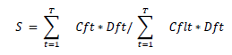
Cft = Fixed Cash flow in coupon period t Cult = Floating Cash flow at coupon period t Dft = Discount factor at coupon period t

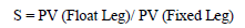
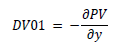
As stated above, Swap pricing is a function of the underlying interest rate, and it directly depends on the shape of the yield curve. If y represents the current yield curve, then MTM (Mark to Market) of the Swap is given by PV(y). It is essential to define the sensitivity of the Swap concerning the interest rate movement for hedging purposes. The use of this sensitivity is to determine the hedge notional. This sensitivity is defined as DV01 or Duration defined as

DV01 = PV (y+1) – PV(y)

Alternatively

Modified Duration is defined as

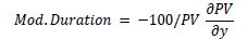
The concept of DV01 or Duration is taken from the fixed income, Bond portfolio management.

The dollar value of a 01 (DV01), also called the present value of 01 (PV01), refers to the change in the value of financial security, such as a bond, for a basis point change of 0.0001 in interest rates. DV01 is measured in the minor dollar change and is not expressed as a ratio or percentage. As a result, DV01 provides investors and analysts with the evolution of a bond's price in dollars based on the 0.0001-point change in its yield to maturity relative to interest rates. Since the primary goal of Hedging is to lock in a bond's present position regardless of any changes in its maturity yield, the paramount for selling or buying a bond's hedge position for every $1 par value is determined by the hedge ratio based on the original position.

The "Effective Duration" of a bond is evaluated in years. It measures the sensitivity of a bond's prices in relation to interest rate fluctuations while considering variables such as final maturity periods in years, yields, calls, coupons, and present values. The risks involved in determining the maturity yield of bonds increase with time due to the negative correlation between interest rates and bond prices. This implies that a fall in interest rates increases the prices of bonds while a rise in interest rates adversely affects bond prices the risks involved in this relationship increase over time. The interpretation of the increase in a bond's Risk as its duration increases is that an investor is compelled to wait for a longer time to recoup their principal investment and yield for a long maturity bond subject to changes in interest rates as compared to a short maturity bond whose price will not fall as much in case of a rise in interest rates.

The "Duration of a Bond" refers to the inverse linear relationship between interest rates and bond prices. The linear relationship is a suitable method of measuring the sensitivity of bond prices to changes in interest rates but only for small yield fluctuations. When bond yield fluctuations are large, the relationship between bond prices and interest rates becomes non-linear, making Duration an unreliable measure of sensitivity. This non-linear relationship for large yield fluctuations is called convexity. A combination of both measures provides a more accurate estimation of the percentage changes in bond prices due to a specific percentage change in bond yield than using Duration alone.

Partial Delta/ Bucketed Delta: In practice, a bond or other fixed-income security including an interest rate swap will often be valued off a yield curve, and we can extend the DV01 and Duration to partial DV01s or critical rate durations - the partial derivatives concerning yields for different parts of the curve:

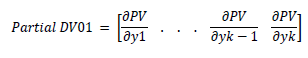
Bucketed delta report is one of the most critical reports an interest rate derivative trader would like to monitor during the day, especially when there is a big swing into the interest rate derivative market. Bucketed delta reports or Key rate exposure reports provide a trader a quick view to place his hedges. A typical Bucketed risk report may look like the following Table 3.

Table 3 Quant.Stackexchange.Com
Risk Buckets	PV01
3 m	-95.39
6 m	26.83
1Y	34.77
2Y	-84.98
3Y	437.65
4Y	84.86
5Y	-83.36
7 Y	-657.40
10Y	-807.02
20Y	-876.69
>20Y	-99.95

Partial Delta report / Bucketed Risk report has become even more critical as the industry is starting to move to a standardized approach of IM (Initial Margin) and VM (Variation Margin), details of the bucketed risk report for the usage of IM calculations can be found in the ISDA methodology document (ISDA SIMM Methodology, 2018).

Financial Market had gone through a turbulent phase during the credit crisis of 2008 (Bernanke, 2009), and as it started receding towards 2010, it taught us some suitable lessons about the Financial Market. One of those was the estimated Libor rates. Historically Libor rates are calculated rates. The post Credit crisis, it was a consensus that Libor could no longer be used as a Risk-free Benchmark rate for the cash flow discounting purpose, and there was a push towards the accuracy of pricing (Justin, 2010). Global Market tend to move towards OIS discounting, and most of the Swaps and OTC Derivatives issued post-credit crisis were valued using the OIS discounting (Hull & White, 2013). Derivative Market moved to a multi-curve framework of curve stripping to preserve the basis (Ametrano & Bianchetti, 2013). Multi-Curve Framework and Dual bootstrapping (Roberto, 2015). Also, the market post-credit crisis has evolved to a great extent. The Clearing of the OTC Swaps was a landmark reform, which also fueled the growth of OIS discounting further as now the swaps started to be fully collateralized. As we moved further, the Market kept innovating itself. Further, the clearinghouses started to allow collateral in a currency that is different from the trade currency; for example, one can enter into a Swap in EUR (Pay Fixed & Receive Euribor 3M); this further complicated the choice of pricing curve, primarily the discount curve as now the discount curve is required to take into account the funding spread arbitrage if the collateral is paid in a currency different than trade currency.

While the pricing became more accurate as the Market started to price Credit risk, Liquidity risk, and funding arbitrage on non-trade CSA (ISDA Protocol, 2014), the representation of interest rate sensitivity in bucketed delta / KRD (Key rate Delta/Duration) became more complex. The dual curve stripping and multi-curve framework of curve generation have made the Risk very complicated, even for a simple plain vanilla Interest rate Swap. CSA discounting added further complexity on the top of it. Since Hedging is one of the primary activities of the traders, it became a concern for the traders to hedge their open positions, which was easy earlier as the hedge recommendation provided by the KRD reports have now Risk scattered all across the places and various instruments making the hedging cost very high. Also, hedges are no longer static as there are multiple basis relations among the various curve instruments that need to be preserved to maintain a target hedge ratio. In the present work, we would like to examine the increase in complexity of the Risk of the simple swaps and their variants in various periods and how the advent of SOFR discounting NYFED ARRC Report 2019.

Literature Review

LIBOR rates are the primary benchmark Index for many developed financial markets. The London Interbank Offered Rate (LIBOR, ICE LIBOR) is the most common benchmark interest rate index series used to adjust many financial instruments and contracts (SIFMA, 2019). The London Interbank Offered Rate, better known as LIBOR, refers to a series of widely used reference rates that underpin interest rates for various financial products. It has grown dramatically since the 1980s to become a reference rate for a significant proportion of financial products globally (UK Finance, 2018). Post credit Crisis Libor Index came under criticism for various manipulations and misreporting to favor the trading position of certain big banks and broker-dealers. LIBOR's volatile behavior during the financial crisis provoked questions surrounding its credibility. Beginning in June 2012, LIBOR came under public scrutiny due to controversy over.

Individual panel bank submissions during the height of the financial crisis. Allegations arose that banks had purposefully underreported their borrowing costs by significant amounts to Project financial strength amidst market uncertainty (Hou & Skeie, 2014). There was a genuine need to find a rate index that can be used as a benchmark rate index in the future and has a feature and potential to replace the Libor index NYFED, 2014. SOFR (Secured Overnight Funding Rate) had features encouraging potential candidates. SOFR has several characteristics that LIBOR and other similar rates based on wholesale term unsecured funding markets NYFED, 2019. NY FED formed an ARRC (Alternative Reference Rate Committee) to find a benchmark rate index in 2014 NY FED User Guide, 2019. This task presumably would be one of the most significant rate migration projects across the entire Capital market (SIFMA, 2019). Many researchers and Market practitioners believe that Libor Cessation will be a benchmark event for the whole of the finance industry. Libor Cessation is a significant milestone for the global capital market (Schrimpf & Sushko, 2018). The London Interbank Offered Rate (LIBOR, ICE LIBOR) is the most common benchmark interest rate index series used to adjust many financial instruments and contracts (SIFMA, 2019).

Libor rates are the primary source of major derivative products. Therefore the OTC Swap constricts and its variant flavors like single currency basis swap, Cross Currency Basis Swap, CMS Swap, etc., are the most widely used underlying instrument to strip the curve (Medvedev, 2018). SOFR, the new benchmark index, will change the curve construction methodologies entirely. Generally, there are two curve construction approaches: bootstrapped curve or a globally solved curve. Several pieces of literature are available, and one such paper is the Bank of Canada working paper series 2000-17 (Uri Ron, 2000). The yield curve offers a valuable set of information for monetary policy purposes. It gauges information about the expected path of future short-term rates and economic activity and inflation (Per Nymad-Anderson, 2018).

Some of the shortcomings reported by ARRC of FED ARRC Report 2018 can be outlined as General Issues: There were general issues in Libor. These issues were creating problems and misinformation in a Derivative Contract. Since Libor is quoted as an estimate and not out of the actual transactions, it is possible to manipulate it, which has happened in the past. In the post-credit crisis, the capital market, especially the Derivative Market, reacted very negatively to the Libor as a benchmark rate index. They are detailing some of those as follows.

Libor Manipulation: Post-credit crisis, there were concerns that Libor could be manipulated. Some of the banks reported lower Libor rates to showcase financials. Also misreported Libor to position their portfolio in profit falsely. This came out as a "Libor Scandal," In June 2012, the CFTC announced a hefty fine against the banks who were actively involved in Libor frauds. Non-Risk Free / Uncollateralized: The benchmark rate should be risk-free during the crisis. Libor being an estimated rate, was uncollateralized. While the economy was good, Libor worked as a reasonable risk-free benchmark. Still, in post-credit turmoil, there was significant default in the Libor based contract in a stretched economic situation, therefore not being collateralized. The financial Market started looking for an alternate index that could be collateralized and considered Risk-free for discounting purposes.

During the post Credit crisis, it was a consensus that Libor could no longer be used as a Risk-free Benchmark rate for the cash flow discounting purpose (Justin, 2010). Global Market tend to move towards OIS discounting, and most of the Swaps and OTC Derivatives issued post-credit crisis were valued using the OIS discounting (Hull & White, 2013). Derivative Market moved to a multi-curve framework of curve stripping to preserve the basis (Ametrano & Bianchetti, 2013). Multi-Curve Framework and Dual bootstrapping (Roberto, 2015). Also, the market post-credit crisis has evolved to a great extent. The Clearing of the OTC Swaps was a landmark reform, which also fueled the growth of OIS discounting further as now the swaps started to be fully collateralized. As we moved further, the Market kept innovating itself, and further, the clearinghouses started to allow collateral in a currency that is different from the trade currency; for example, one can enter into a Swap in EUR (Pay Fixed & Receive Euribor 3M), this further complicated the choice of pricing curve primarily the discount curve as now the discount curve is required to take into account the funding spread arbitrage if the collateral is paid in a currency different than trade currency. A complication of Risk arises from the difficulty of construction of pricing curves of a swap (discount Curve, Forecast curve). Curve construction is done with a particular set of objectives & constraints (Hagan & West, 2008). Some of them are:

Curve construction criteria: Curve instrument should be most liquid with the tightest bid/ask spread. For this reason, usually, a yield curve instrument is chosen to be Money market instruments, Futures, Swaps, Basis Swaps, etc., depending on their liquidity in the Market. Port Credit Crisis when Market moved to OIS discounting, OIS outright swaps are liquid only till 2 years of maturity, so to extend the curve further, Libor-OIS (Fed Fund) basis swaps need to be developed further be added on the longer end of the curve.

An interpolation scheme to be chosen such that hedges are as localized as possible. A spilled Risk in a non-risk bucket creates artificial exposure and hedging issues. Forwards need to be arbitrage-free, which also essentially means that forwards need to be positive. Also, forwards need to be smooth. Patrick Hagan and Graeme West have tabulated the interpolation schemes that work on the abovementioned criteria Figure 3.

Methodology

As outlined in the objective section, we have boxed the KRD report into four-time buckets below Figure 4.

We took the following set of Swaps as our working portfolio and computed the risk / DV01 to compute a KRD / Bucketed risk report finally Figure 5.

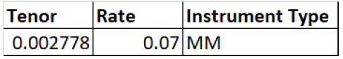
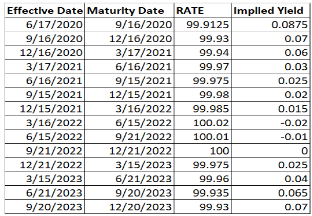
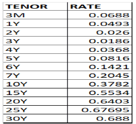
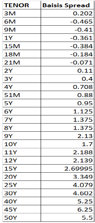
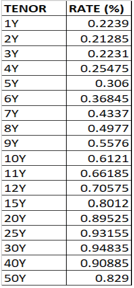
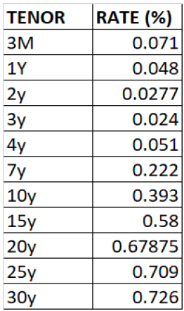
As mentioned in the first Curve construction criteria in the Literature section, we must have the most liquidly quoted curve instruments in the Market. For this reason, a yield curve instrument is usually chosen to be Money market instruments, Futures, Swaps, Basis Swaps, etc., depending on their liquidity in the Market. After the Credit Crisis, when the Market moved to OIS discounting, OIS outright swaps were liquid only until two years of maturity. To extend the curve further, Libor-OIS (Fed Fund) basis swaps need to be developed further to be added on the longer end of the curve. Therefore, the Curve instrument was no longer the same in similar curves across those 4-time boxes. As mentioned, the choice of the underlying mechanism depends on the liquidity of that instrument. Various curves in the defined time boxes may differ (Bloomberg, 2012). For example, the pricing curves [Discount Curves & Forecast Curve] for a Plain vanilla USD swap are as follows in the first three-time boxes Figure 6.

The above choice of instruments in the curve has been supported in very literature Fabio Mercurio (2018) and more generally in the writings of Quants in the front office pricing and risk systems like Numerix (Dan, 2013), Bloomberg (Mercurio, 2012) & Open Gamma (Marc Henrard, 2018).

Now that we have our curve structure and the actual curve has been generated using the conventional methodologies described in various literature, including but not limited to Bianchetti's paper (Ametrano & Bianchetti, 2013) and the SOFR curves as defined by Fabio Mercurio (Mercurio, 2018) we have generated our yield curve (Details in the appendix section) defined we take our stylized Swap and try to compute the Risk and KRD/ Bucketed Risk report. Our Sample Swap confirms is shown below Table 4.

Table 4 Summary Of Our Example Swap Confirm
Term Sheet Summary
Notional	10,000,000
Currency	USD
Fixed Coupon	0.3060%
Par Swap Rate	0.3060%
Swap MTM	0.00
Swap Maturity	5Y
Swap Owner	Pay Fixed
Counterparty	Pay Float
Floating Index	Libor 3M
Spread	0 bps
DV01	$ 4,760.00
Payment Frequency	3M (Quaterly)

This is a 5Y swap with a notional of 10 Million USD, with an effective 24^th August 2020. It is struck at Par (Fixed coupon is equal to the 5Y par Swap rate). Since it is struck at par, the NPV (Swap MTM – Mark to Market) is equal to zero though it has a genuine interest rate sensitivity of $4760. It is a quarterly payment swap where the swap owner (Counterparty 1) is paying a fixed par rate (0.306%) and receiving Libor 3M (with no spread on the floating leg). We calculated the Risk of this Swap in all the time boxes. The results are shown below Figure 7.

In time box 1, the Risk is distributed in a Base Libor curve concentrated on a 5Y bucket as expected (Localness property of the curve construction), in time box 2, the Risk is distributed across Libor 3M Base curve and Libor OIS basis curve which is complicated than what we see in the time box1. In time box 3, the Risk is distributed across Libor 3M base curve and SOFR discount curve, which is a bit more complicated than time box 1 but simpler than time box 2. Time box 4 refers to the period when Libor cessation has already taken place, so no risk has been shown in time box 4. For trading and hedging purpose, vanilla swap is cheaper and more transparent than basis swap. Therefore, we can conclude that if we can put the KRD (Key Rate Duration) report in the scale of complexity, the following order holds good for the Plain Vanilla Interest Rate Swap.

KRD (Key rate Duration) can also be computed using PCA-Principal Component Analysis (Kumar, 2022). PCA is a basically reducing the dimensionality of the data (Roland et al., 2021).

Note on valuation and curve calibration: For the swap pricing purpose, the curve is calibrated as suggested in research papers Amertrano & Bianchetti. For the SOFR turn, we resort to Fabio Mercurio's work (Mercurio, 2018). Minor differences in the calculation of DV01 can be attributed to the following.

1. Curve instruments are different in all the time boxes, and the differences stem from optimization error. The tolerance of our optimization algorithm (Levenberg-Marquardt) was set to $1 for a 1 M (1000,000) Notional, and one can observe that our sample trades have 10M USD as the notional difference is less than $10, which explains the difference.

2. As a rule of thumb in the derivative Market, this difference is acceptable.

As mentioned in the introduction section, the KRD report suggests a set of hedge trades to make the portfolio Delta Neutral / DV01 Neutral (Immune to Interest Rate Risk), so in the case of Time Box 1, the trader needs to enter into the following Trade to make the Swap (or a portfolio of Swap) delta neutral.

TB 1

1. Single Trade of 5Y Receive Fix and pay Floating Libor 3M with DV01 close to USD 4760.

TB2

2. One Trade of 5Y Receive Fix and Pay Floating Libor 3M with a DV01 of USD 4880.14
3. Second Trade of 5Y pay the basis with the Basis Spread 01 of USD 112.59

TB3

1. One Trade of 5Y Receive Fix and Pay Floating Libor 3M with a DV01 of USD 4365.12
2. One trade of 5Y with Pay SOFR1D and Rec Fixed coupon with equivalent SOFR DV01 of USD 412.24.

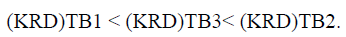
Implications for Sell-side Market participants: As a rule, the execution cost of the Plain Vanilla interest rate swap is less than that of a basis swap Trade web, TCA 2020. Also, plain Vanilla interest rate Swap is supported by most of the Electronic SEFs (Swap Execution Facility), which reduces the operational overhead. It reduces the TCA (Transaction Cost Allocation), making Swap execution cheaper. In contrast, all the electronic SEFs do not support basis swaps. A big chunk of those basis swaps is traded on Voice/ Phone/ Bloomberg Chat, which incurs operational overhead in processing and settlement, resulting in a higher TCA for Basis swap. Therefore, we can say that the TCA in time box 2 is higher than the TCA of time box three, higher than the TCA of time box 1. Therefore, we can also put it on a scale as (TCA) TB1< (TCA) TB3< (TCA) TB2. Thus we can conclude that hedging cost, which was lower in the pre-credit crisis era, went up in the post-credit crisis, but the advent of SOFR discounting has reduced the cost of Hedging. This cost of Hedging will further go down with Libor cessation as we will then move to the one SOFR curve world (Just like one Libor curve world in the pre-credit Crisis timeframe.

Implication for Buy-Side Market Participants: Buy-side firms will also be impacted similarly with SOFR, but they have another cost of operations. As per the regulation, most buy-side firms need to get their portfolio valued daily by a third-party fund service provider. These fund service providers provide pricing services to these buy-side firms. These firms are IHS MARKIT, Thompson Reuters Valuation service, Bloomberg BVAL, Hedge Serve, etc. On average, they charge somewhere around 25-40 cents to value a Swap position in the standard market scenario and approximately 50-60 cents per basis swap. Therefore, in the Time Box 2 situation, this hedge fund would incur the highest valuation service bill to those valuation service providers.

Therefore, we can arguably conclude that with SOFR discounting, the risk representation and Hedging cost would go down for both sell-side and buy-side market participants. They will be positively impacted by the “Risk rationalization of OTC Derivatives in SOFR transition.”
For other Swap variants, too, as captured in the literature review, the pricing curve [Set of the Discount curve & Forecast Curve] will determine the complexity of the Risk. As we have noted, as the curve dependency and interlink age between the pricing curve in terms of basis spread increases, the risk bucket also increases because now the curve instrument and therefore Risk attributable buckets have gone up, giving rise to the complexity and cost of hedging multi-fold. In the tables below, we would like to share with our reader an idea of how the pricing curve assignment and their dependencies/ basis increase and the Risk. Once again, we will examine the increasing complexity of curve assignment in those four-time boxes. Time Box 1: Pre-Credit Crisis (2009 & Before) Figures 8 to 11.

Future Research (Each Point to be Written in Detail)

This section will cover some aspects of SOFR that need further lookup & research that have not been researched thoroughly yet. Some of them are:

Development of Non-linear Market in SOFR: Since SOFR discounting and SOFR Index switch is a new and unexplored area for non-linear products. CME has started clearing SOFR Mid-curve options, but the OTC market is rater unknown, and we feel that it is a good area of further research as we progress towards the Libor cessation around the first quarter of 2022.

When we create a curve for the discounting purpose, we tend to include the most liquid instrument available. When we move to the full SOFR world, there will be an issue of convexity adjustment in curve construction as the more extended SOFR contracts are geometrically compounded. In contrast, the shorter tenured contracts will be compounded (Arithmetic compounding), giving rise to convexity as both types of instruments will be needed in the curve, and the angle needs to be calibrated in the presence of both types of compounding (Takada, 2011). This will be an additional convexity term in the curve calibration apart from the convexity adjustment due to the future presence.

In a related topic of convexity adjustment for the money market future instruments. Since Future instruments are an integral part of the curve construction and convexity needs to be adjusted for curve calibration, there is still a search for volatility for SOFR based index. Though CME has just started publishing SOFR options, money market volatility for SOFR is still very sparse, and this can be a good topic to work on.

One more challenge in Curve construction is turn rate impact on the curve. Usually, towards the year-end or around the financial reporting time, the demand for liquid money market instruments shoots up as every company wants to add liquidity in their finance/ balance sheet reporting. This creates a short-lived "Flight to Quality" (Vayanos, 2004) situation giving rise to the price of Money market instruments. This price rise makes a jump in the curve as money market instruments are generally included in the curve in the short end region. While this inclusion of turn rate is researched and well implemented by many industry quants (Ametrano & Bianchetti, 2013), this area is unexplored from the SOFR curve construction perspective and a good area for further research.

Conclusion

Like turn rate, FOMC meeting dates also produce a kink in the curve. The FOMC holds eight regularly scheduled meetings during the year, which directly impacts the interest rate. No specific literature exists explaining the handing of the possible kink in the SOFR curve and how to resolve this in the interpolation of forwards.

Appendix (Data)

SOFR Curve data (08/24/2020)

SOFR money market rate

SOFR Futures

SOFR Swaps

Fed fund-SOFR Basis Swap

Base libor swap

OIS (Fed fund Swap)

Libor sofr basis swap

References

Ametrano, F.M., & Bianchetti, M. (2013). Everything you always wanted to know about multiple interest rate curve bootstrapping but were afraid to ask. Available at SSRN 2219548.

Indexed at, Google Scholar, Cross Ref

Bernanke, (2009). Firefighting: The Financial Crisis and Its Lessons.

Indexed at, Google Scholar, Cross Ref

Bloomberg, (2012).  Extending USD OIS Curves using Fed Fund Basis Swap Quotes.

Google Scholar, Cross Ref

California Debt & Investment advisory Commission, (2007) https://www.treasurer.ca.gov/cdiac/publications/math.pdf

Google Scholar, Cross Ref

Dan, L. (2013). Numerix, Dilemmas in the Multi-Curve Approach.

Google Scholar, Cross Ref

Financial Crisis Inquiry Commission report, (2011). Official Government Edition January 2011.

Google Scholar, Cross Ref

Hagan & West, (2008). Methods of Constructing a Yield Curve, Wilmott Magazine 2008.

Indexed at, Google Scholar

Hou, D., & Skeie, D. (2014).  LIBOR: Origins, Economics, Crisis, Scandal, and Reform, Federal Reserve Bank of New York Staff Reports.

Indexed at, Google Scholar, Cross Ref

Hull &White, (2013). The fva debate. Journal of Investment Management, 11(3), 14-27.

Indexed at, Google Scholar, Cross Ref

ISDA SIMM Methodology, (2018). ISDA Publications for SIMM Calculations.

Justin, C. (2010). http://janroman.dhis.org/finance/OIS/Edu-Risk/Swap%20Discounting%20And%20OIS%20Curve.pdf

Kumar, S. (2022). Effective hedging strategy for us treasury bond portfolio using principal component analysis. Academy of Accounting and Financial Studies Journal, 26(2), 1-17.

Google Scholar

Lin, Markwardt & Zhang, (2014). Deriving Economic Impacts of Derivatives, Milken Institute publications.

Indexed at, Google Scholar, Cross Ref

Mercurio, (2018). A Simple Multi-Curve Model for Pricing SOFR Futures and Other Derivatives SSRN 3225872.

Indexed at, Google Scholar, Cross Ref

Michael, C. (1994). BIS Quarterly review. https://www.bis.org/ifc/publ/ifcb35a.pdf

Indexed at, Google Scholar, Cross Ref

Per Nymad & Anderson. (2018). ECB Statistics Paper Series No 27, February 2018.

Indexed at, Google Scholar, Cross Ref

Roberto, B. (2015). A Note on Dual-Curve Construction: Mr. Crab's Bootstrap, Applied Mathematical Finance, 22(2).

Indexed at, Google Scholar, Cross Ref

Roland, G., Kumaraperumal, S., Kumar, S., Gupta, A., das, Afzal, S., & Suryakumar, M. (2021). PCA (Principal Component Analysis) Approach towards Identifying the Factors Determining the Medication Behavior of Indian Patients: An Empirical Study. Tobacco Regulatory Science, 7(6-1), 7391-7401.

Google Scholar

Schrimpf, A., & Sushko, V. (2019). Beyond LIBOR: a primer on the new benchmark rates. BIS Quarterly Review March.

Indexed at, Google Scholar

SIFMA, (2019). Insights: Secured Overnight Financing Rate (SOFR) Premier, July 2019.

Google Scholar,

Takada, (2011). Valuation of Arithmetic Average of Fed Funds Rates and Construction of the US dollar Swap Yield Curve.

Indexed at, Google Scholar, Cross Ref

UK Finance, (2018). Discontinuation of LIBOR – UK Finance guide for business customers.

Google Scholar

Uri Ron, (2000). A Practical Guide to Swap Curve Construction, Bank of Canada Working Paper 2000-17.

Indexed at, Google Scholar

Vayanos, (2004). Flight to Quality, Flight to Liquidity, And the Pricing of Risk, Working Paper 10327, National Bureau of Economic Research.

Indexed at, Google Scholar, Cross Ref

Received: 27-Jan-2022, Manuscript No. AAFSJ-22-11000; Editor assigned: 29-Jan-2022, PreQC No. AAFSJ-22-11000(PQ); Reviewed: 14-Fab-2022, QC No. AAFSJ-22-11000; Revised: 17-Mar-2022, Manuscript No. AAFSJ-22-11000(R); Published: 24-Mar-2022