Keywords

Equity, Risk, Return, Trade Volume, Portfolio, Risk Surprise.

Introduction

The most prevalent asset pricing models, regardless of the factors they involve, are cross-sectional analyses to describe relationships. Since the broad adoption of Markowitz’s (1952) pioneering work in modern portfolio theory, the asset pricing studies focus on decomposing risk factors to explain return, implicitly assuming that risk and return move in the same direction. Most recently, McLean & Pontiff (2016) deliver a mega study summarizing the previous papers, showing that stock returns are predictable in cross-sectional regressions with 97 variables identified in the literature.

However, in the practice of asset selection and portfolio management, practitioners frequently encounter numerous assets that carry high volatility but deliver poor returns. Otherwise, there are also a great number of assets, with high Sharpe ratios, that realize excellent capital gains without high levels of volatility. The occurrence of the incongruity is so frequent that simply using market anomaly as an explanation seems to be inadequate. In fact, an earlier study by Dong & Guo (2019) prove that risk and return of equity assets do not comove from a time-series standpoint.

Cejnek & Randl (2016) decompose ex ante risk premia embedded in the dividend derivative pricing, thereby, identifying substantial return time variation, independent from risk. This indirect evidence shows that asset risk and returns, from a time series perspective, is not necessarily correlated. A similar study in the commodity futures market demonstrates that there is no comovement of contemporaneous or intertemporal risk and return regarding the prices of crude oil futures (Gong et al., 2017). This implies that the phenomena of risk-return independence are not limited to the equity market. Dong & Guo (2019) explore such independence without identifying any fixed risk effect. This research thus continues to decompose the asset risk levels into the expected risk and risk surprise, and attempts to explore if risk surprise plays a role in explaining asset returns.

Existing literature reconciles the risk and return deviation from two perspectives: redefining the methods of measuring and representing risk and return; and identifying factors that cause the deviation of risk and return.

In the first perspective, researches focus on criticizing and adjusting the methods of measuring and representing risk and return. The main point is that risk and return are still positively correlated regarding time series analyses; and any violation of the relationship is due to biased measurements. Ganzach (2000) suggests that this explains the need for redefining risk among familiar and unfamiliar assets. Daniel et al. (2018) conclude that asset prices comprise, not only the priced risk associated with the factor loadings, but also unpriced risk that is measured, but not represented. Wang et al. (2017) use the risk adjusted return (RAR) and attempt to support the conventional risk return relationship. Londono-Yarce & Xu (2019) differentiate between the behaviors of downside and upside variance risk premia in the U.S. market, and suggest asymmetric return compensations. Baba Yara et al. (2018) suggest that return variation, due to common value, is associated with standard proxies for risk premia, but contrary to models that exclusively generate a value premium in equities.

Related to the second perspective, researches focus on identifying factors that cause the deviation of risk and return. The main point is that the risk-return independence is due to certain market failure, mainly caused by behavioral motivations. Piccoli et al. (2018) suggest that the conflict is explained by investor sentiment, as the relationship between conditional variance and stocks return is negative in periods of high sentiment. Fiegenbaum & Thomas (1988) find a negative risk-return association for firms with returns below target levels. They suggest that this is consistent with the basic propositions of prospect theory. Theodossiou & Savva (2016) show that this is because of negative skewness in the distribution of portfolio excess return. Bonomo et al. (2015) explain the risk-return contradiction at short and long horizons, by proposing an asset pricing model with generalized disappointment aversion preferences.

Among these arguments, there is a lack of investigation that uses broad range dataset to quantify the market sentiment introduced by risk. In other words, sentiment, caused by investor surprises, are only limited to their return terms but should be extended to the risk terms. Therefore, the time series relationship between return, expected risk, risk surprise, and volume, is a meaningful gap in literature that warrants a separate investigation, suggested by Bali & Zhou (2016) and supported by Baba (Yara et al., 2018).

Our research reviews the relationship among expected risk, unexpected risk, return, and trade volume from the time series perspective, including the lagged values of these variables. This is inspired by the suggestion provided in Asness et al. (2019):

“To further test the link between the price and return to quality, it is interesting to exploit the time-variation in the price of quality…The time series of these cross-sectional regression coefficients reflects how the pricing of quality varies over time.”

Peng (2016) also takes such initiative and compares the performance of the index-based time series and the cross-sectional approach in exploring factor loadings of nontraded assets.

We use the constituents of the Russell 3000 Index to perform the test of the impact of risk surprise. With these 2,797 stocks, we use AR (1) models to fit each of their monthly risk time series to obtain the regression specification. Each AR (1) model produces a time series of risk surprise, or unexpected risk, as the residual of the projected current risk, based on the previous term risk level. Such risk surprise is employed to examine its impact on the current and future return and trade volume levels.

By using the time series return data of the Russell 3000 constituents, we minimize the incomparable liquidity and credit risk premium. Our study provides evidence that if an asset has an influential previous risk level, then a higher unexpected risk at the prior period will significantly decrease the current asset return. However, trade volumes of assets are related to multiple factors, and risk surprise is not an adequate explanation. Most often, among the significant regressions, the current trade volume increases with higher current unexpected risks, and decreases with higher lagged unexpected risks.

Our results are consistent with the findings of Lee & Li (2016), which uses a nonparametric regression approach and shows that idiosyncratic risk is negatively related to returns at the low quantiles. A study by Bollerslev et al. (2015) demonstrates that the variance risk premium can be used to predict future market returns, and the same pattern is specified in Table 1. They conclude that the market fears play an important role in understanding the return predictability. Further, we find that the market return is less explained by investor actions regarding the trade volume.

In addition, Bowen & Hutchinson (2016) use the U.K. data and draw similar conclusions to ours. Whitelaw (2000) studies the connections between risk and return in a general equilibrium exchange economy. The findings show a complex, non-linear and time-varying relation between expected returns and volatility. Such nonlinearity inspires our motivation to explore the different layers of risk components.

The rest of this paper is organized as follows: section 2 explains the data processing and sampling methods employed to obtain a comparable set of regression observations; section 3 summarizes the AR(1) regressions conducted to obtain the unexpected risk on the data series of each of the 2,350 equities in the test pool, as well as the 447 equities in the robustness check pool. In section 4, we report the regression results and their implications in terms of the risk residual and return reaction. Section 5 concludes and suggests the topics to address in the future.

Data and Sampling

The goal of our study is to test the relationships among the equity return, risk surprise, and trade volume. We are including numerous publicly traded equity assets listed on different security exchanges, to ensure that our conclusion is not biased, related to equity size, value factor, or industry representations. Also included is an extremely long time series of transaction records, to minimize the impact of business cycle and macroeconomic policies. However, we do not incorporate the assets that are less liquid, because the stale transaction price can lead to smoothed and therefore undervalued risk.

We select the Russell 3000 Index constituents, a commonly used representative sample set in the U.S. equity market. The holdings of this index represent a balanced spectrum of equity across size, value type, and industries. A significant number of studies in the past decades use it to represent a broad and balanced equity pool, for example, (Coggin et al., 1993; Chaney & Philipich, 2002; Guerard et al., 2018).

The Center for Research in Security Prices (CRSP) provides the adjusted closing equity price variable used in our study. The daily returns of equity calculated from this variable are free of the impact from dividend distributions, splits, and reverse splits. We include equities that carry a history of longer than 420 daily returns to ensure that there are at least 20 monthly standard deviations to perform the AR (1) regressions. This leaves us with 2,797 equities. The start point of the dataset is from January 2, 1950, or since the IPO, whichever was earlier. The end point of the dataset is February 14. 2019. We used a fixed-width window of 21 trading days to obtain the standard deviations of returns at the monthly level. This serves as proxy of monthly risk of the assets. Additionally, we convert the daily returns and volumes into 21-day returns and volumes, as proxy.

We adopt the 21-day window rather than the normal calendar month in this study for significant reasons. Firstly, it is the average number, 252 trading days in a year; secondly, the different number of days in a normal calendar month makes the comparison of the monthly-level standard deviations from daily return data less legitimate; and lastly, monthly return, volatility, and volume data are less affected by random trade noises and market surprises driven by investor sentiments.

The monthly returns, risks, and volumes of trade of an asset i in month τ are calculated with the equations below:

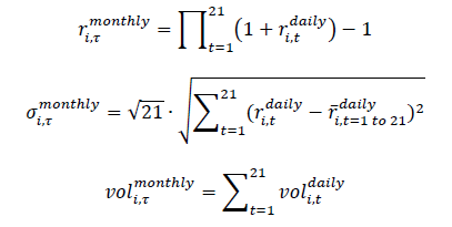
In the equations, the variable 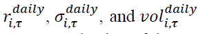are the daily return, risks, and volume of an asset i on day t. τ. Due to our selection of the monthly window, the monthly returns are not consistent with the calendar-based monthly returns. Therefore, in our study, the start and end of each month are not limited to the beginning or the end of the calendar months, but keep the same criteria of 21 days. This also mitigates the month-of-the-year effect, such as the well-known January effect (Reinganum, 1983). To moderate the data-mining concern caused by this 21-day window framework, we set up robustness tests to verify the reliability and consistency of our results. In these tests, we use a randomly selected start date to summarize the regression relationships among risk, return, and trade volume. The selection of start date is not important, since the fixed 21-day window will make the subsequent windows start with very scattered and irregularly distributed dates.

For the 2,797 publicly traded equities, we use the first 2,350 to form the test pool of result summary, then use the remaining 447 to form the robustness check group for cross examination. The equities are sorted alphabetically by their trade tickers. The robustness check group is separated by an independent regression summary comprising the last 350 equities on the list. This method avoids the concern of robustness check group selection bias in terms of equity size, value, liquidity, or other factors. In other words, the robustness check group is generated randomly.

We use the following criteria for the selection and setup of the test group and the robustness check group, by maintaining more than 80% of the equities from our sample in the test group, so that we can produce representative and reliable conclusions. To ensure that there are more than 400 equities to form the robustness check group, we bring a meaningful portfolio from each industry, size, and value groups. The results reported in Section 4 provide evidences that there is no significant difference between the test group and the robustness check group.

Regression Summary Methodology

The major work of our study is to summarize the regressions for each of the 2,350 stocks from the test group, and compare the summary with the one concluded from the robustness check group on its 447 equity components. The AR (1) regressions performed for each equity:

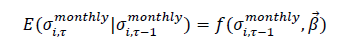
And the AR (1) regressions performed for each equity, in their model specification forms, are:

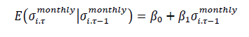
And the risk residuals, also named unexpected risk or risk surprise in this study, is defined as:

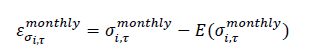
Simply put, the risk residuals are the difference between the forecasted current risk based on the AR (1) model regression coefficients and the realized risk, by combining the new returns realized at the market place.

Our paper focuses on the interaction of the risk, return, and the volume variables. We summarize the percentage of regressions performed on equities with significant coefficients at 5% level, as well as the signs of the coefficients. The magnitudes of the 2,797 regression coefficients are available upon request. We do not report the average regression coefficients, since the average coefficients are meaningless, except for their signs, in forecasting the risk-return or volume-return relations. There are 1,742 regressions from the test group that have significant β1; There are 350 regressions from the robustness check group that have β1 that are meaningful. The proportions are 74.13% and 78.30%, respectively. This implies that the current risk levels of approximately three out of four stocks are significantly affected by their previous risk levels.

Specifically, we perform the following regressions on the risk residuals obtained from the 1,742 regressions and 350 regressions in both groups.

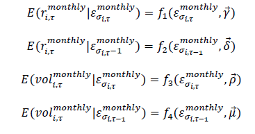
The 4 regressions above aim to answer the following three main questions: (1) if the risk surprise defined in our study is a meaningful measure; (2) how the risk surprises affect the current asset returns and future asset returns; (3) how the risk surprises affect the current asset trade volume and future asset trade volumes.

Results

Tables 1and 2 report the main findings of our study. We first perform the time series regressions of the risks of the 3,000 equities regarding their lagged risks. There are 2797 valid regressions that we adopt in this study, and we exclude 203 regressions due to insufficient daily returns to produce monthly risks that carry a history long enough to run a time series regression. Specifically, an individual stock must have at least 421 daily prices to produce 420 daily returns used to generate 20 monthly risks. Further, any equity that fails to produce 20 monthly risks is not included in the risk variable time series regressions.

Table 1 The Impacts of Current and Lagged Risk Residuals on the Equity Returns
Regression Functions	Test Group (1742 significant regressions)			Robustness Check Group (350 significant regressions)
	Total number of significant regressions	Negative Impact	Positive Impact	Total number of significant regressions	Negative Impact	Positive Impact
Return=f(current risk residual)	778	471	307	156	95	61
	44.66%	60.54%	39.46%	44.57%	60.90%	39.10%
Return=f(lagged risk residual)	1029	1017	12	216	212	4
	59.07%	98.83%	1.17%	61.71%	98.15%	1.85%

 

Table 2 The Impacts of Current and Lagged Risk Residuals on the Equity Trade Volumes
Regression Functions	Test Group (1742 significant regressions)			Robustness Check Group (350 significant regressions)
	Total number of significant regressions	Negative Impact	Positive Impact	Total number of significant regressions	Negative Impact	Positive Impact
Trade Volume=f(current risk residual)	750	6	744	166	2	164
	43.05%	0.80%	99.20%	47.43%	1.20%	98.80%
Trade Volume=f(lagged risk residual)	272	213	59	58	47	11
	15.61%	78.31%	21.69%	16.57%	81.03%	18.97%

We then divide the 2797 equities that support the monthly return standard deviation calculation into two groups: test and robustness check. The test group includes randomly selected 2350 stocks; the remaining 447 stocks are categorized in the robustness check group. The equities in both groups vary in size, value, and industry identities.

In the test group, a total of 1,742 (74.12%) stocks have relationships between their current risk and lagged risks, thus supporting our notion of risk residual. In the robustness check group, a total of 350 (78.30%) stocks have a correlation between their current risk and lagged risks. In general, the risk levels of a majority of the equities are affected by the lagged risk levels.

The risk residuals, which are the unexpected risks calculated from the AR(1) regressions of risks, are then used to test their explanatory power on asset returns and trade volumes. We find that 45% of the time, the current unexpected risks affect the current asset returns, whereby, 61% of them decrease the returns and 39% of them increase the returns. However, the lagged unexpected risks affect the current asset returns 60% of the time, and most of the significant impacts are negative. This implies that if an asset has an influential previous risk level, then a higher unexpected risk at the prior period will significantly decrease the current asset return. In other words, asset returns do not increase with risk, but do the opposite. Higher risk surprises from the previous term suppress the current term returns.

Related to trade volume, we find that less than 50% of the current unexpected risks and approximately 16% of the lagged unexpected risks substantially affect the current trade volume. This implies that the transaction activities at the microstructure level are related to a broad spectrum of factors beyond risks. However, among the significant regressions, almost all the time, higher current unexpected risks increase the current trade volume, and higher lagged unexpected risks decrease the current trade volume. Higher unexpected risk triggers and amplifies the current trade activities, but discourages the future density of transactions.

In both sets of tests regarding the asset returns and trade volumes, the results are highly consistent between the test group and the robustness check group. This is due to the random identification of assets between the two groups based on the alphabetic orders of asset tickers, and the random definition of the start day of the 21-day windows used to generate monthly risks and monthly trade volumes.

Concluding Remarks

This paper uses the constituent of the Russell 3000 Index to perform the test of the impact of risk surprise. We first exclude 203 stocks in the index component pool because they have fewer than 421 daily prices on the record to support the creation of 20 monthly risk observations. With the 2,797 stocks, we use AR(1) models to fit each of their monthly risk time series to obtain the regression specification. Each AR(1) model produces a time series of risk surprise, or unexpected risk, as the residual of the projected current risk, based on the previous term risk level. Such risk surprise is employed to examine its impact on the current and future return and trade volume levels.

We find that if an asset has an influential previous risk level, then a higher unexpected risk at the prior period will significantly decrease the current asset return. However, trade volumes of assets are related to multiple factors and risk surprise does not have overwhelming explanatory power. However, among the significant regressions, almost all the time, higher current unexpected risks increase the current trade volume, and higher lagged unexpected risks decrease the current trade volume.

This paper, while confirming the existence and the impact of risk surprise, raises a set of questions: the cause of the delayed reaction of asset returns upon a realized risk surprise; the cause of faster reaction of trade volume than asset return; and the cause of the dispersed current return reaction on risk surprises. There are number of plausible explanations. For example, the slow information flow is caused by transaction cost and research cost; and the increasing trade volume is triggered by a mix of long-term investors and mean-reversion investors, and so on. However, more evidences are needed to support these hypotheses, and we leave the research of them to future studies.

References

1. Asness, C., Frazzini, A., & Pedersen, L. (2019). Quality minus junk. Review of Accounting Studies, 24(1), 34-112.
2. Baba Yara, F., Boons, M., & Tamoni, A. (2018). Value timing: risk and return across asset classes. SSRN Electronic Journal.
3. Bali, T., & Zhou, H. (2016). Risk, Uncertainty, and Expected Returns. Journal of Financial and Quantitative Analysis, 51(3), 707-735.
4. Bollerslev, T., Todorov, V., & Xu, L. (2015). Tail risk premia and return predictability. Journal of Financial Economics, 118(1), 113-134.
5. Bonomo, M., Garcia, R., Meddahi, N., & Tédongap, R. (2015). The long and the short of the risk return trade-off. Journal of Econometrics, 187(2), 580-592.
6. Bowen, D., & Hutchinson, M. (2014). Pairs trading in the UK equity market: risk and return. The European Journal of Finance, 22(14), 1363-1387.
7. Cejnek, G., & Randl, O. (2016). Risk and return of short-duration equity investments. Journal of Empirical Finance, 36, 181-198.
8. Chaney, P., & Philipich, K. (2002). Shredded Reputation: The Cost of Audit Failure. Journal Of Accounting Research, 40(4), 1221-1245.
9. Coggin, T., Fabozzi, F., & Rahman, S. (1993). The Investment Performance of U.S. Equity Pension Fund Managers: An Empirical Investigation. The Journal of Finance, 48(3), 1039-1055.
10. Daniel, K.D., Mota, L., Rottke, S., & Santos, T. (2018). The cross-section of risk and return. Columbia Business School Research Paper, 18-4.
11. Fiegenbaum, A., & Thomas, H. (1988). Attitudes toward Risk and the Risk-Return Paradox: Prospect Theory Explanations. Academy of Management Journal, 31(1), 85-106.
12. Ganzach, Y. (2000). Judging risk and return of financial assets. Organizational Behavior and Human Decision Processes, 83(2), 353-370.
13. Gong, X., Wen, F., Xia, X.H., Huang, J., & Pan, B. (2017). Investigating the risk-return trade-off for crude oil futures using high frequency data. Applied Energy, 196, 152-161.
14. Guerard, J.B., Markowitz, H., Xu, G., & Wang Z. (2018). Global portfolio construction with emphasis on conflicting corporate strategies to maximize stockholder wealth. Annuals of Operations Research, 267(1), 203-219.
15. Lee, B.S., & Li, L. (2016). The idiosyncratic risk-return relation: a quantile regression approach based on the prospect theory. Journal of Behavioral Finance, 17(2), 124-143.
16. Londono-Yarce, J.M., & Xu, N.R. (2019). Variance Risk Premium Components and International Stock Return Predictability. SSRN Electronic Journal.
17. Markowitz, H.M. (1952). Portfolio selection. The Journal of Finance, 7(1), 77-91.
18. McLean, R.D., & Pontiff, J. (2016). Does academic research destroy stock return predictability? Journal of Finance, 71(1), 5-32.
19. Peng, L. (2016). The Risk and Return of Commercial Real Estate: A Property Level Analysis. Real Estate Economics, 44(3), 555-583.
20. Piccoli, P., da Costa, N.C.A., da Silva, W.V., & Cruz, J.A.W. (2018). Investor sentiment and the risk-return tradeoff in the Brazilian market. Accounting and Finance, (S1), 599-618.
21. Reinganum, M.R. (1983). The anomalous stock market behavior of small firms in January: Empirical tests for tax-loss selling effects. Journal of Financial Economics, 12(1), 89-104.
22. Theodossiou, P., & Savva, C.S. (2016). Skewness and the relation between risk and return. Management Science, 62(6), 1598-1609.
23. Wang, Y., Qiu, Z., & Qu, X. (2017). Optimal portfolio selection with maximal risk adjusted return. Applied Economics Letters, 24(14), 1035-1040.
24. Whitelaw, R.F. (2000). Stock market risk and return: an equilibrium approach. Review of Financial Studies, 13(3), 521-548.