Keywords

Simulation Model, Markov Chains, BCG Matrix, Steady State Probabilities

Introduction

Simulation is a methodology that is applied to learn about a real system, prototyping a model based on the system. It allows exploring different aspects and although it is not an optimization technique, it helps to propose possible solutions to different system scenarios, contributing to decision making (Carson, 2003; Ceballos, Betancur Villegas & Betancur Villegas, 2014; Pulido-Rojano, De la Hoz-Reyes & Melamed-Varela, 2017; Pulido-Rojano, Sanchez Sanchez & Melamed Varela, 2018). Simulation is also seen as an applied methodology that allows modeling and acquiring knowledge about the behavior of complex environments, which are often difficult to interpret when they are approached analytically (Hillier & Lieberman, 2015). Its application covers areas such as the product design and development, inventories, stochastic systems analysis, waiting lines analysis, financial processes, health systems, among others (Chakravarthy & Rumyantsev, 2020; Heredia Acevedo, Fernando Ceballos & Sanchez Torres, 2020; Ozdemir & Kumral, 2019; Baril, Gascon & Vadeboncoeur, 2019; Riquelme, Gatica & Orozco, 2015).

When proposing a simulation model, it must be considered that there are input variables that can be controllable and others that are not controllable (probabilistic) (Law, 2006). Generally, controllable variables are defined before running the model, however, the probabilities are generated randomly to interact in the model and observe the results of this interaction (see Figure 1) (Anderson, Sweeney, Williams, et al., 2019). One of the most important uses of simulation models is that they allow analyzing the possible results of a system by voluntarily changing the input values of the controllable variables and thus, giving recommendations about how the real system should operate (Forero de Lopez, 2019; Hillier & Lieberman, 2015). Although simulation is not applied as an optimization method, it helps to describe or predict how a system will work with options given for controllable data and values that are obtained at random considering historical data. This to achieve desirable systems, designed to function according to the desired characteristics (Pulido-Rojano & García-Díaz, 2018).

Source: Adapted from Anderson, Sweeney, Williams, et al., (2019)

Simulation models are divided into continuous models and discrete models. The difference is that continuous models deal with systems that change continuously over time and discrete models deal with systems where changes in their state occur instantaneously at random or specific points in time because of the occurrence of discrete events. In general, most of the known models obey simulations by discrete events; moreover, there are adapted models where it is possible to approximate continuous changes in the state of the system by means of discrete events (Rabe, Deininger & Juan, 2020).

This document proposes a novel simulation model for predicting the behavior of products or business in the market, applying the Markov chains and The BCG classification Matrix. The Markov chains is a special type of discrete stochastic process in which the probability of an event occurring depends only on the immediately preceding event. It’s used to observe and analyze the evolution of one variable over time (Including products) until obtaining the future probabilities of the states of it (Jensen, Jerez & Valdebenito, 2020). Meanwhile, the BCG matrix is a graphical classification method that helps to carry out a strategic analysis of a company's products portfolio, based on two dimensions: the market growth rate and the relative participation rate. As a strategy tool, it serves to understand the strategic position of the business portfolio, recognize the best and worst products, promote the right investment, among others (Malhotra, 2016). The model proposed in this document aims to classify products according to its growth rate and relative participation rate, using the BCG matrix, to calculate the probabilities of transition from one classification to another using the concepts of Markov chains by simulations and thus, obtain the steady state probabilities of the product over time. This will allow any company to propose a set of strategies or actions based on simulations of the future behavior of the product that bring it to a desired classification status. A step-by-step algorithm was also designed to display the model instances and it was validated by a case study that involved the use of real data for a specific product. The combination of the Markov processes and the BCG matrix has not yet been addressed and the goal is to create a simulation model that can be reproduced and used by companies that want to make decisions based on the predictions of their products behavior. It should be noted that currently the most used models to predict products behavior are based on sales forecast models and the life cycle model, therefore, a new prediction approach based on the BCG matrix and the Markov chains offers a novel alternative for portfolio management.

This document is structured as follows. Section 2 presents a theoretical summary of the BCG matrix. Section 3 describes the Markov chain process. Section 4 presents the MARKOV- BCG simulation model. Section 5 shows the results and analysis of the numerical experiments and finally, section 6 presents the conclusions of the present investigation.

Growth-Participation Matrix (BCG Matrix)

Companies seek constant growth and be competitive, they want their products or services to please and satisfy their customers, and at the same time, to maintain growth in participation and profitability in the market. For this reason, organizations use some models that help them to somehow classify their brand and see if the strategies used are ideal or see how the behavior of their product or service would be (Ramirez Hassan, García Peláez & Garcés Ceballos, 2011; Kotler & Keller, 2015). Market research and analysis techniques are very useful in providing information that allows reducing the uncertainty about the behavior and reactions that a product will have when it is put on the market, analyzing the elements and variables that interact in the environment to make tighter decisions (Fernández Nogales, 2004; Malhotra, 2016).

The BCG Matrix is a business portfolio model developed and proposed in the 1970s by the American consulting firm Boston Consulting Group (BCG). It is one of the most significant classification techniques developed by strategic management for multiproduct companies. It is based on a two-dimensional analysis to graph and categorize the different products or businesses into four categories depending on their levels of growth and profitability (see Figure 2). The BCG matrix classifies each product or business in one of the four quadrants known as: Cash Cows, Stars, Question Marks and Dogs. The interpretation is that the products or businesses, with different levels of growth and profitability, located in each of these quadrants, will be in positions of cash requirement, which leads to some implications on how the company should build its portfolio (Olivares Ramírez, Huesca Chávez & Contreras Jiménez, 2011).

Source: Adapted from Ramírez Hassan, García Peláez & Garcés Ceballos (2011)

According to Ramírez Hassan, García Peláez & Garcés Ceballos (2011); David & David (2017), the description of each product or business is directly related to the position it occupies in the classification, for example:

• Stars: They are products or businesses with high levels of growth that generate a high volume of income. These have positive cash flows and require high investment to maintain their relative leadership position. Generally, once the product reaches maturity it becomes a "Cash Cows" business.

• Cash Cows: They are products or businesses that have a relatively large share of the market but compete in a slow-growing industry. They are cash generators because they produce money above their needs. Many of today's "Cash Cows" were "Stars" yesterday. These businesses seek to maintain their strong position as much as possible.

• Question Marks: They are products or businesses that occupy a relatively small position in the market but compete in a high growth industry. Generally, these products require a lot of investment, but generate little or no cash. These businesses are called question marks because the organization must choose whether to reinforce them through some intensive marking strategy that will take them to a "Star" category or simply give up on them before becoming a "Dog" product.

• Dogs: These businesses have low relative participation and compete in an industry with little or no market growth. Due to their weak internal and external position, these businesses are often liquidated or discarded. Generally, their behavior requires that the little cash flow they generate be reinvested in the operation of the business.

As we can see, the specific position of each product will depend directly on the Relative Participation Rate (PR) and the Growth Rate (GR) of the products in the market. The PR is obtained from the ratio or index of dividing the sales of the company's product or business in the market in a particular industry by the sales of the product or business of the most important rival company in that industry (see equation (1)).

Where, VE are the sales of the company’s product or business in a specific period and VC are the sales of the product or business of the largest competitor in the same period.

For its part, the Growth Rate (GR) is obtained as the percentage of growth in sales of the company's product or business from one period to the next and it can be calculated as shown in equation (2).

Where VE₁ is the sales of the company's product or business in period 1 and VE₂ are the sales of the company's product or business in period 2. For the cases of product classification through the BCG matrix, the ranges of values of each quadrant are determined as follows:

Markov Chains

In probability theory, a special type of discrete stochastic process in which the probability of an event occurring depends on the immediately preceding event is known as Markov chain or Markov model. This memoryless feature is called the Markov property (Valenzuela, Rojas & Hjalmarsson, 2018). A Markov chain is a tool that represents a system that varies its state over time, each change being a transition of the system. A discrete-time system X={Xn : n ≥ 0} is said to form a Markov chain if the probabilities of its possible j state in the period n + 1 (P(X_n+1)) depend exclusively on the probabilities of its i state in the immediately previous period (P(X_n)) and not from the previous periods (X_n-1, X_n-2,…,X₀), i.e., P(X_n+1=j | X_n=i) ∀ n. That is, if we have the present information from the system, knowing how it got to the current state does not affect the probabilities of moving to another state in the future. These probabilities, known as transition probabilities, are contained in a matrix P of dimensions |S| × |S| with P=(p_ij) i,j ∈ S. As we can see, the changes are not predetermined, but the probability of the next state is based on the previous one, said probability is homogeneous over time (Carreño-Sanchez & Sanabria- Codesal, 2019). Mathematically, the expression that would represent the calculation of the future state of any of the states of the system will be given by equation (3).

where X_n ∈ R_p is the probability vector of the i states at time n ∈ N and P ∈ R_p is the transition probability matrix between the states, which meets three conditions:

1. each state probability in time n + 1 depends exclusively on the previous state n, that is, it is a first-order difference equation,

2. the transition probability matrix (P) has all its inputs greater than or equal to zero, i.e., p_ij=P(X_n+1=j |X_n=i) ≥ 0; ∀ i, j ε S and,

3. the sum of the elements of each row of the matrix P is equal to 1, that is, ∑_j∈S p_ij=1.

Considering the above, the solution of the system is also given by equation (4).

Where Pⁿ is the nth power of the matrix P and X₀ is the probability vector of the states in the initial period. Also, expression (4) can be demonstrated as follows:

In this way, the probabilities of the states in a period n can be calculated using the matrix P at its nth power. Also, the long-term steady-state probabilities of the system can be calculated, i.e., when n tends to infinity (n →∞). In these cases, the probabilities of the matrix P will

remain unchanged or in a state of equilibrium and it is only necessary to perform the product of matrices up to a value considerably far from n or to solve the system of equations starting from equation (3) (see Anderson, Sweeney, Williams, et al., (2019) for more information). States in a Markov chain are defined as a characterization of the situation in which the system finds itself at a given instant. These states are defined as finite when there are a defined number of states in the system (Sánchez-Brenes, Alvarado-Ulloa, Solís-Blanco, et al., 2016). Some of the applications of the Markov chains include, for example, weather forecasting, genetic inheritance analysis, Inventory, prediction of daily fluctuations in stock prices, among others (Pasricha, Selvamuthu, D’Amico et al., 2020; Yun, Qin, Yang, et al., 2019; Zhang & Schmöcker, 2019; He & Jiang, 2018).

Markov-BCG Simulation Model

The proposed simulation model (which we will call the MAR-KOV-BCG Model) is based on the fact that if we have the probabilities of transition of a product or business between its possible states (State 1 (S1): Cash Cows, State 2 (S2): Stars, State 3 (S3): Question Marks or State 4 (S4): Dogs), we could use Markov processes to predict their future behavior. For this, historical sales data of the company's product and historical sales data of the product of the largest competitor in the industry would be used to estimate the probability distribution of sales and thus, obtain the Growth Rate (GR) and Participation Relative (PR) in the simulation periods. These sales values will be the probabilistic entries of the MARKOV-BCG Model and will serve to simulate the behavior of the product states in the market. The deterministic entries will be the possible number of product states and the classification scales of each state according to the BCG Matrix (see Table 1). The objective is to construct the matrix of transition probabilities (P) between the states considering the change of state of the product from one period n to the next n

+ 1 and to study its behavior over time (see Figure 3).

The logical algorithm associated with the MARKOV-BCG model contains the following steps:

• Step 1: Select the product or business to simulate considering that there are historical product sales data and historical product sales data from the largest competitor in the industry.

• Step 2: Establish the product states (State 1 (S1): Cash Cows, State 2 (S2): Stars, State 3 (S3): Question Marks or State 4 (S4): Dogs) and the values of the classification scale according to the BCG matrix (Table 1).

• Step 3: Determine the probability distribution of product sales of the company and the probability distribution of product sales values of the largest competitor in the industry.

• Step 4: Generate the random values of the sales of the company and its biggest competitor for N simulation periods and calculate the N values of the Relative Participation (PR) and the N - 1 values of the Growth Rate (GR). Note that the GR can only be calculated from the N=2 period of the simulation.

• Step 5: Determine the product status according to the BCG Matrix from the coordinates obtained from the GR and the PR from period N=2 to period N.

• Step 6: Obtain the frequencies of the change from each state of the product from one period to the next and construct the transition probability matrix P using the relative frequencies of the changes produced. Note that the first change in product status occurs from period 2 to period 3, therefore, N - 2 changes will occur throughout the simulation. Also, it must be considered that the product can remain in the same state (i=j) from one period to the next.

• Step 7: Calculate the steady-state probabilities from the transition matrix P.

In this way, we can use the Markov chains concept to create a transition matrix P that allows us to analyze the probability of occurrence of the product classifications in a BCG matrix. This model has been little studied and simulation through the interaction of the BCG matrix and the Markov processes has not yet been addressed. This gives greater importance to this document, showing a way to study the behavior of products for effective decision making.

Results and Analysis

As a first step in validation of the MARKOV-BCG model presented in the previous section, historical data were taken from the last 20 periods (months) of a service provided by a company in the city of Barranquilla (Colombia). This sample was obtained through a non- probabilistic convenience sampling, where the company voluntarily agreed to supply data on the sales of its service. In this case, data was obtained on the number of users who received the service per period. Likewise, using the same sampling method, it was possible to obtain the number of users of this same service from the largest competitor (see Table 2). Due to confidentiality restrictions, the companies in this case study did not want to reveal their names or offer information about their sales in monetary units. However, the information collected was useful enough to validate our model. Step 2 asks to define the possible states of the product during the simulations according to the values of PR and GR, which correspond to the quadrants of the BCG matrix presented in Table 1 and Figure 2.

Table 1 Product Classification Values in the BCG Matrix
Product	PR	GR
Stars	Greater than 1	Sales growth greater than 10%
Cash Cows	Greater than 1	Growth in sales less than or equal to 10%
Question Marks	Less than or equal to 1	Sales growth greater than 10%
Dogs	Less than or equal to 1	Growth in sales less than or equal to 10%

Table 2
Historical Sales Data
Period	Sales in number of users (VE)	Sales in number of users of the largest competitor (VC)
1	649	767
2	620	845
3	641	601
4	594	840
5	640	1007
6	648	638
7	698	924
8	680	915
9	734	866
10	679	807
11	715	624
12	670	933
13	674	930
14	658	929
15	736	890
16	725	682
17	603	842
18	638	910
19	742	617
20	730	711

Table 3 Distribution Fit Test For The VE and VC Sales Variables
Distribution	VE	Log Likelihood	Distribution	VC	Log Likelihood
	Parameters			Parameters
Uniform	2	-99,9442	Uniform	2	-120,127
Gamma	2	-104,289	Smaller Extreme Value	2	-123,568
Normal	2	-104,298	Weibull	2	-123,692
Birnbaum-Saunders	2	-104,301	Normal	2	-124,618
Inverse Gaussian	2	-104,301	Gamma	2	-125,086

As step 3, Table 3 shows the summary of the distribution fit test results for the sales variables VE and VC. The data shows the different probability distributions to which the variables can be adjusted and the Log Likelihood statistic. As we can see and according to the Log Likelihood statistic, the distribution that best fits the variables VE and VC is the uniform distribution X~U(a=Lower limit, b=Upper limit) with parameters U(a=594, b=742) for VE and U(a=601, b=1007) for VC. In this way, by knowing what type of distribution the variables follow, we can simulate the sales values as a probabilistic input to the model and calculate the GR and PR values. Also, possible N-1 product classifications can be identified. Table 4 presents the summary of the application of the MARKOV-BCG model for an N=120 months (Steps 4 and 5). As an example, Figure 4 also shows the first 20 product classifications based on Table 1 during the application of the simulation model.

Table 4 Results of the Simulation of the Markov-BCG Model for N=120
N	Values generated for VE	Values generated for VC	PR	GR	State
1	659	1098	0,60
2	691	879	0,79	4,86%	Dog
3	610	892	0,68	-11,72%	Dog
4	680	712	0,96	11,48%	Question Mark
5	722	686	1,05	6,18%	Cash Cow
6	625	680	0,92	-13,43%	Dog
7	692	768	0,90	10,72%	Question Mark
8	647	760	0,85	-6,50%	Dog
9	670	883	0,76	3,55%	Dog
10	616	835	0,74	-8,06%	Dog
.	.	.	.	.	.
.	.	.	.	.	.
.	.	.	.	.	.
111	668	913	0,73	-14,25%	Dog
112	659	850	0,78	-1,35%	Dog
113	640	620	1,03	-2,88%	Cash Cow
114	695	841	0,83	8,59%	Dog
115	633	740	0,86	-8,92%	Dog
116	623	972	0,64	-1,58%	Dog
117	696	611	1,14	11,72%	Star
118	703	953	0,74	1,01%	Dog
119	629	922	0,68	-10,53%	Dog
120	631	904	0,70	0,32%	Dog

Table 5 contains the frequencies of the changes between the 4 possible states of the product from one period to the next (Step 6). The values were obtained considering the initial state of the product in a given period n and its state in the following period n+1, for example, if the product started in S1 (Cash Cows) during a period, the number of times the product remained in the same state (i=j) in the following period was equal to 3. Likewise, the changes to S2 (Stars), S3 (Question Marks) and S4 (Dogs) were equal to 0, 4 and 10, respectively. During the simulation, N - 2 changes between states were recorded, which correspond, in our case, to 120 - 2=118 changes in total.

Table 5 Frequency of Changes Between States
	Cash Cows (S1)	Stars (S2)	Question Marks (S3)	Dogs (S4)
Cash Cows (S1)	3	0	4	10
Stars (S2)	2	0	0	3
Question Marks (S3)	3	0	0	12
Dogs (S4)	9	5	11	56

Table 6 shows the transition probabilities p_ij between the 4 possible states, calculated from the frequencies in Table 5. For example, in the case of calculating the probability of transition between S1 (Cash Cows) and S4 (Dogs), this was obtained by dividing the frequency in Table 5 by the total number of changes produced starting from S1 (Cash Cows), that is, 10/17

= 0.5882. This calculation procedure guarantees that all the sums of the transition probabilities per row are equal to 1 (Σ_j∈S p_ij=1), which is a necessary condition in a Markov chain. In this same way, the remaining probabilities between the states were calculated.

Table 6 Transition Probability Matrix (P)
	Cash Cows (S1)	Stars (S2)	Question Marks (S3)	Dogs (S4)
Cash Cows (S1)	0.1765	0.0000	0.2353	0.5882
Stars (S2)	0.4000	0.0000	0.0000	0.6000
Question Marks (S3)	0.2000	0.0000	0.0000	0.8000
Dogs (S4)	0.1111	0.0617	0.1358	0.6914

Finally (Step 7), starting from equation (3), it was possible to establish the system of equations to be solved to calculate the stable state probabilities of the product in each state (see from equation (6) to (10)). Note that when considering the stability of the system when n tends to infinity (n → ∞), we can say that there will be no change in the probabilities between the

periods n and n + 1. In this way, the system of equations to solve for our case will be given by the following expressions.

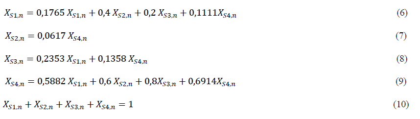
Table 7 presents the steady state probabilities calculated for the product after solving the system of equations. As observed, the probabilities that the product remains in each state when n ® ¥, are: X_S1,n=14,41%, X_S2,n=4,24%, X_S3,n=12,71% and X_S4,n=68,64%. These probabilities give a clear idea of what state the product will be in overtime and promote the design of appropriate strategies to bring the product to a state that generates profitability for the company. As we can see, the highest percentage of the time the product will remain in the “Dogs” State, so the company must intervene to change the current conditions of the product in the market, until it reaches a point where the highest long-term probabilities are found in S1 (Cash Cows) or S2 (Stars). Marketing theories claim that the products “Dogs” are products whose relative market share is weak, with very low sales and margins in a declining sector. Furthermore, they operate at a productive disadvantage with very few opportunities for growth at a reasonable cost. The most common recommendations include bringing the product to a specialized segment of the market, protecting it from incursions by any hostile competition. Also, it is recommended to find a way to reduce its different costs and support its cash flow.

Table 7 Steady State Probabilities Of The States For
	Cash Cows (S1)	Stars (S2)	Question Marks (S3)	Dogs (S4)
Cash Cows (S1)	0,1441	0,0424	0,1271	0,6864
Stars (S2)	0,1441	0,0424	0,1271	0,6864
Question Marks (S3)	0,1441	0,0424	0,1271	0,6864
Dogs (S4)	0,1441	0,0424	0,1271	0,6864

Conclusions

We have presented the design of a simulation model that considers a combination of the principles of the Markov processes and the BCG Matrix. The model is a novel methodology that allows predicting the behavior of products or businesses in the market, helping to make decisions in business. A logical algorithm was designed for its implementation, considering the controllable input variables and the probabilistic variables. The model was validated using historical data on the sale of a service from a company and its largest competitor. The implementation of the model included determining the probability distribution of the sales data, the classification of the product from one period to the next according to the BCG matrix, the calculation of the transition matrix and the calculation of the steady state probabilities. The model aims at deepening the product analysis, since the BCG matrix is generally used only as a tool in the marketing area to classify the lines of growth and participation of a product, without predicting its behavior. The results of the numerical experiments confirm the efficiency of the model in predicting the behavior of product states in the long term. As a relevant aspect, the proposed model not only aims to classify the product or business, but to predict, through simulations, the permanence that the product or business will have in each classification. Also, considering that the most used methods to predict the behavior of products in the market are based on forecasting methods and the life cycle of the product. In this way, organizations will be able to make decisions that take their product to a desirable position. Likewise, the present study intends to become a frame of reference for future studies on this topic. Future research should continue to study different types of products with a greater range of portfolios, comparing and studying their evolution from sales data in physical and monetary units. Also, a set of market strategies based on product evolution during simulation experiments could be designed for each classification range, probability values, and product type.

Acknowledgment

This paper is a product of the project entitled: "Metodología para la predicción de los comportamientos de los productos o servicios en el mercado aplicando la matriz BCG y los procesos Markovianos" financed by Universidad Simón Bolívar, Barranquilla, Colombia.

References

1. Anderson, D.R., Sweeney, D.J., Williams, T.A., Camm, J.D., Cochran, J.J., Fry, M.J., & Ohlmann, J.W. (2019). Fundamentals of Quantitative Methods for Business (13th Edition). México D.F.: Cengage Learning.
2. Baril, C., Gascon, V., & Vadeboncoeur, D. (2019). Discrete-event simulation and design of experiments to study ambulatory patient waiting time in an emergency department. Journal of the Operational Research Society, 70(12), 2019-2038.
3. Carreño-Sanchez, A., & Sanabria-Codesal, E. (2019). Analysis of social networks using Markov chains. Modelling in Science Education and Learning, 12(1), 21-30.
4. Carson, J.S.I.I. (2003). Introduction to modelling and simulation. Proceedings of the 2003 Winter Simulation Conference, 7-13.
5. Ceballos, F., Betancur Villegas, J.P., & Betancur Villegas, J.D. (2014). Discrete simulation applied to health care models. Research and Innovation in Engineering, 2(2), 10-14.
6. Chakravarthy, S.R., & Rumyantsev, A. (2020). Analytical and simulation studies of queueing-inventory models with MAP demands in batches and positive phase type services. Simulation Modelling Practice and Theory, 103.
7. David, F.R., & David, F.R. (2017). Strategic management concepts. México D.F.: Pearson.
8. Fernández Nogales, A. (2004). Research and market techniques. Madrid: ESIC Editorial.
9. Forero de Lopez, G. (2019). Research and innovation in engineering for a sustainable world-4.0. Research and Innovation in Engineering, 7(1), 4-5.
10. He, Z., & Jiang, W. (2018). A new belief markov chain model and its application in inventory prediction. International Journal of Production Research, 56(8), 2800-2817.
11. Heredia Acevedo, D., Fernando Ceballos, Y., & Sanchez Torres, G. (2020). Event simulation model discrete for the analysis and improvement of the customer service process. Research and Innovation in Engineering, 8(2), 44-61.
12. Hillier, F., & Lieberman, G. (2015). Introduction to operations research. México D.F.: McGraw - Hill Interamericana.
13. Jensen, H.A., Jerez, D.J., & Valdebenito, M. (2020). An adaptive scheme for reliability-based global design optimization: A Markov chain Monte Carlo approach. Mechanical Systems and Signal Processing, 143.
14. Kotler, P., & Keller, K.L. (2015). Marketing management (15th Edition). México D.F.: Pearson.
15. Law, M.A. (2006). How to build valid and credible simulation models. Proceedings of the 38th Winter Simulation conference, 58-66.
16. Malhotra, N. (2016). Market research: Essential concepts. México D.F.: Pearson.
17. Olivares Ramírez, G.M., Huesca Chávez, J.A., & Contreras Jiménez, J.C. (2011). Business strategy models and designs. Contributions to the Economy.
18. Ozdemir, B., & Kumral, M. (2019). Simulation-based optimization of truck-shovel material handling systems in multi-pit surface mines. Simulation Modelling Practice and Theory, 95, 36-48.
19. Pasricha, P., Selvamuthu, D., D’Amico, G., & Manca, R. (2020). Portfolio optimization of credit risky bonds: A semi-Markov process approach. Financial Innovation, 6(1). https://doi.org/10.1186/s40854-020-00186-1
20. Pulido-Rojano, A., De la Hoz-Reyes, R., & Melamed-Varela, E. (2017). Advances in operations research and management sciences. Barranquilla, Colombia: Simón Bolívar University editions.
21. Pulido-Rojano, A., Sanchez Sanchez, P., & Melamed Varela, E. (2018). New trends in operations research and administrative sciences: An approach from Ibero-American studies. Barranquilla, Colombia: Simón Bolívar University Editions.
22. Pulido-Rojano, A., & García-Díaz, J.C. (2018). Simulation and improvement of the multihead weighing process. Proceedings of Seventeenth Ibero-American Conference on Systems, Cybernetics and Informatics (CISCI), 58-63.
23. Rabe, M., Deininger, M., & Juan, A.A. (2020). Speeding up computational times in simheuristics combining genetic algorithms with discrete-Event simulation. Simulation Modelling Practice and Theory, 103.
24. Ramírez Hassan, A., García Peláez, S., & Garcés Ceballos, J.D. (2011). Changes in the market position of Colombian companies. Economic Semester, 14(30), 37-59.
25. Riquelme, P., Gatica, G., & Orozco, E. (2015). Design of an operation model for urban transport routing based on discrete simulation. Research and Innovation in Engineering, 3(2), 1-12.
26. Sánchez-Brenes, A., Alvarado-Ulloa, C., Solís-Blanco, R., Chacón-Cerdas, R., & Villalta-Solano, H. (2016). Application of Markov Chains in an invitro plant production process. Technology in March Magazine, 29(1), 74-82.
27. Valenzuela, P.E., Rojas, C.R., & Hjalmarsson, H. (2018). Analysis of averages over distributions of Markov processes. Automatica, 98, 354-357
28. Yun, M., Qin, W., Yang, X., & Liang, F. (2019). Estimation of urban route travel time distribution using Markov chains and pair-copula construction. Transport metrics B, 7(1), 1521-1552.
29. Zhang, C., & Schmöcker, J.D. (2019). A Markovian model of user adaptation with case study of a shared bicycle scheme. Transport metrics B, 7(1), 223-236.