Research Article: 2022 Vol: 26 Issue: 1
Study of the Performance of Machine Learning Algorithms in the Case of Islamic Stock Market
Kaoutar Abbahaddou, Mohammed V University in Rabat
Mohammed Salah Chiadmi, Mohammed V University in Rabat
Citation Information: Abbahaddou, K., & Chiadmi, M.S. (2022). Study of the performance of machine learning algorithms in the case of islamic stock market. Academy of Accounting and Financial Studies Journal, 26(1), 1-12.
Abstract
This article analyzes the performance of Machine Learning models in the prediction of stock market indices returns. The empirical study is based on the case of Islamic stock market. The accuracy rate will be the tool used to measure the ability of the models to predict the next price and sharpe ratio will be used to evaluate the performance. As a result of this study, we can say that support vector machine (SVM) outperforms other models namely CART, RF and ANN.
Keywords
Islamic Finance, Stock Price Prediction, Machine Learning Algorithms.
Introduction
One of the biggest challenges for financial players is predicting future stock market trends. In fact, it is difficult to make the right investment decisions, given that the market can be extremely volatile. Besides, we can find theories like the Random Walk which is directly linked to the theory of market efficiency, stipulating that the stock price fluctuates randomly. Therefore, it implies that there is no trend governing its evolution, which makes its trend impossible to predict (Akar & Güngör, 2012).
It is in this uncertain environment that investors are constantly looking for new investment solutions, capable of predicting market trends with a great precision, to meet their primary objective, namely the maximization of earnings and returns.
At the same time, artificial intelligence is getting a lot of attention, especially machine learning, that is developing strongly in many areas and seems to offer remarkable results explaining its rise. Financial players will therefore begin to take an interest in it, seeing it as a potential solution to prediction problems. In this article, we will go through the literature. After, we will see machine learning methods in order to finally, study and compare the performance of different algorithms, both in terms of predictions and return. The analysis will be done empirically on the Islamic market case before reporting results and findings.
Literature Review
Stock market investing is getting a lot of attention. In addition, today we have a large amount of information available and public. Therefore, all these data are the basis of the new challenge of understanding and interpreting them in order to seize more investment opportunities in a noisy and dynamic market environment.
Before going through the different approaches adopted for prediction, it is interesting to ask whether we can really have a predictive character, in an environment where the market is said to be efficient. This latter term refers to a market where the information is completely and instantly reflected in the price, with the assumption of no arbitrage opportunity. In that sense, Fama is distinguishing three types of market efficiency. The weak efficiency hypothesis where the historical share price is directly reflected in its price, the semi-strong efficiency hypothesis where public information and the historical price are reflected in the price and finally, the strong efficiency hypothesis where private information, in addition to the information mentioned above, are reflected in the price. Many studies have been carried out on this subject, like Gray & Kern in 2009 or Duan et al. (2009), that question the theory of efficient markets and tell us that markets can become inefficient.
Regarding the study of the performance of financial stock indexes, this can be done with different approaches like the sentiment, technical or fundamental analysis. It consists of predicting the performance of a stock index based on the idea that the stock price follows trends, sometimes cyclically, which helps determine the movement of stock prices. These methodologies are generally based on different data such as lowest prices, highest prices and volume and has been widely used, but also widely criticized. In the sense of the weak form of efficient markets, where the historical price is directly reflected in the share price. Today, different tools are used to try to predict the stock price, based on historical prices and the volume of the traded stocks like the Machine Learning (ML), which has experienced a boom
in its use and application to automation problems in various fields. Specifically in the market finance, we note the presence of studies analyzing the behavior and predictions of stock prices and index variations, involving Machine Learning algorithms. We can also see intelligent trading systems to better predict the evolution of prices under different situations and conditions (Boutaba et al., 2018).
As a matter of fact, Machine Learning is a sub-branch of artificial intelligence that refers to a set of methods and algorithms that allow machines to discover and learn patterns, without receiving programming instructions. For this self-learning to take place, machines need large databases on which to practice and learn independently. Machine Learning will thus be able to draw relationships, links from these masses of data without needing human support. The more data there is, the more efficiently machine learning can be exploited.
There are two learning methods. We can have a supervised learning when the data and the associated solutions are provided to the algorithm. During the learning process, the algorithm will try to find and deduce the relationships between the explanatory variables and the explained variables (label). The algorithm will be executed on a learning base containing examples already covered. Labels can be continuous values (in the case of regression problems) or discrete categories (in the case of classification problems). Some algorithms, such as decision trees, can be used to solve classification and regression problems, while linear regressions can only solve regression problems. Yet, for unsupervised learning algorithms, they are designed to discover hidden structures in a dataset without labels. In this case, the desired outcome is unknown. These include clustering and dimension reduction algorithms.
Another fundamental distinction of machine learning is at the output level. In a classification algorithm, the objective is to find a relationship function between the input data and the discrete output variable. In the case of regression, the output variables will be continuous. Take the example of classifying future movements in the price of a stock. The classification algorithm could have two discrete output variables, 1 if the stock price increases and -1 if the stock price decreases. While the regression algorithm will provide continuous percentage changes in the price of the share as its output (Shah, 2007).
Today, and more than ever, predicting the stock price is becoming an increasingly popular field, especially among artificial intelligence specialists who attempt to create intelligent trading systems. In 2018, Macchiarulo, carried out an analysis based on the S&P 500, where the algorithms were trained on monthly historical data ranging from January 1995 to December 2005, and then apply them over a 10-year trading period as well, until December 2016. In this article, the author first used support vector machines to determine market direction, and neural networks to determine the actual prices and returns of stocks. The two algorithms will then be combined to obtain a prediction that was compared to 20 other strategies. As a result, the Machine Learning algorithm achieved the highest average monthly return at 1.19% and it is the only strategy with an average above one percent. For decline periods, the Machine Learning model outperformed again with an average of 4.12%. It is followed by the strategy based on the fundamental analysis, then the Buy & Hold strategy, with returns of around 3%.
Other studies attempt to verify whether Machine Learning algorithms can contradict the hypothesis of market efficiency, and therefore outperform a Buy & Hold strategy, which would appear to be the best strategy under the assumption that the prices follow the Random Walk theory. This is particularly the case with the study by Skabar & Cloete, from 2002, where a neural network is trained, using a genetic algorithm to try to predict the signals to buy and sell. The time window covers five years, from July 1, 1996 to June 30, 2001. The author compared the returns of four financial price series with the returns obtained on random market data derived from each of these series using a bootstrapping procedure. The four indices considered are the Dow Jones Industrial Average, the Australian All Ordinaries, the S&P500 and the NASDAQ. These sets contain the same distribution of daily returns as the original series. The results show that some financial time series are not entirely random, and that a trading strategy based only on historical price can achieve better returns than a Buy & Hold strategy.
On the other hand, we can find that many ML models studies include technical and fundamental indicators in their analysis. The study of Emir et al. (2012), measures and compares the performance of SVM and MLP (Multi-Layer Perceptron) models and for that they relied on technical indicators and fundamental variables. The study was carried out on the ISE 30 Index (Turkish index) over the period of time from 2002 to 2010. 12 technical indicators were used as variables in the models, as well as 14 fundamental indicators. The results obtained highlighted the performance of the SVM model. Indeed, whether it is technical or fundamental variables, this model performs better than the Multi-Layer Perceptron. The authors also compared the contribution of variables and it seem that the two models with fundamental analysis offer more promising results than the models with technical indicators. A double comparison was therefore done in this study, at the level of the models and the variables to be considered, and put forward the SVM algorithm, and the fundamental indicators.
Another study that compares the performance of ML algorithms to financial indicators is the one of Yan, Sewell & Clack, from 2008. They were interested in portfolio optimization, using machine learning, technical analysis and genetic programming (a sub-branch of artificial intelligence) and focused their study on the Malaysian market. A comparison was therefore made between Support Vector Machines (SVM), Standard Genetic Programming (SGP) and the Moving Average Convergence Divergence indicator (MACD) where the objective was to visualize which method offered the best return on investment over a period of time. from July 31, 1997 to December 31, 1998. In this case, the SGP outperforms the other two strategies, offering more profitable results (1%). The MACD, although offering a negative ROI, nevertheless outperforms the Machine Learning SVM model. Whether it is SVM or MACD, the strategies have a negative Sharpe Ratio, therefore implying that the returns are too low for the risk considered.
We can therefore see that results differ from one study to another. However, despite the increasing importance of Islamic finance over years, we can find only few empirical studies on this area that mostly focus on the comparison of the performance of Islamic Indexes to the common ones. For instance, Hussein in 2004, tested and showed that the returns of FTSE Global Islamic Index perform similarly comparing to FTSE All-World Index. In 2005, he showed also that the monthly returns of FTSE Global Islamic index and Dow Jones Islamic Market Index over perform statistically on short period and on the long run comparing to their common index over a 9 years period. Therefore, giving the differences in ML models performance results and the scarcity of studies on the Islamic stock market. We will focus our research on comparing the performance of ML algorithms with an empirical analysis on the Islamic stock indexes.
Data and Methodology
In order to compare the performance of different Machine Learning algorithms, we used two Islamic stock market indices:
1. Morgan Stanley Capital International Islamic (MSCII), launched in March 2007 and covering 69 countries.
2. Jakarta Islamic Index (JKII), launched in 2000 and focused on 30 companies of foods production and distribution.
3. The implementation of the machine learning algorithms is done on R.
Data Preparation
We collected first the daily historical data over a ten-year period, from January 4, 2010 to January 2, 2020 and it contains six following variables for each specific date. Namely, the opening price (Open), the highest trading price (High), the lowest trading price (Low), the closing price (Close), the quantity of shares traded (Volume) and finally the adjusted price at the close of a date, taking into account the distribution of dividends (Adj.Close).
Several challenges were encountered in the data collected such as the existence of outliers and missing values due mainly to weekends and holidays or even technical and human errors. Thus, in order to harmonize our dataset, depending on the case, we either replaced these values with an average or delete these instances. A third approach is also available and it is about the prediction of these values using machine learning models such as the K nearest neighbor method.
Next, we defined the independent variables on which our machine learning models rely to make their predictions. Using the data already collected, we constructed three variables. The first variable corresponds to the difference between the opening price and the closing price for the same period. The second represents the difference between the highest price and the lowest price over that period. Finally, the last variable measures the difference between the volume traded the next day and the volume traded the same day. This last variable cannot be calculated for the last date of our sample. This line is then deleted.
The dependent variable (Y) corresponds to the label attached to our data that the model tries to predict on the basis of the independent variables. In our case, this variable defines whether the following day's stock price will close up or down and take either the value 1 or the value 0. In order to do this, we calculated returns based on the Adjusted closing price. Based on that, we were able to create the variable that takes 1 if the return is positive and 0 if the return is negative. The last row in the database was deleted because it was not possible to calculate the yield on that date, nor the difference in volume.
Separating the dataset is an essential step in building a machine learning model. The objective is to divide the database into two parts: the first part is used by the model to train and try to discover links between our three explanatory variables and our explained variable, and the second part is used by in order to attempt to predict the dependent variable, namely the label, on the new data. The more data we afford to the algorithm to learn, the more it will provide an accurate model. Therefore, we decided to use 80% of the data as training data, and 20% to test the model.
Implementation of Machine Learning models
Four different supervised algorithms were used for this analysis:
Classification and Regression Tree (CART)
The first model developed is a Classification And Regression Tree (CART), which is a decision tree algorithm that always begins with a root, extended by branches designating the decision rules. We then end up with internal nodes, which represent characteristics, to arrive to the leaves that correspond to the results. This is a strictly binary algorithm and has two branches for each node of the tree. CART is easy to interpret and provides an overview in organizational chart form. This algorithm uses the Gini index to determine which attribute the branch should be generated. This index therefore measures the degree of inequality for a variable, on a given sample. The goal is to choose the attribute that will make the minimal Gini index after dividing the node. This index is measured as follows:
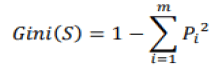
Where S is representing the set, the node contains m classes and pi is the relative frequency of class i in the set S. If ?? is pure, then (S)= 0. Therefore, the higher the index is, the weaker the knot is considered pure. However, CART is not suitable for very large databases and although its performance has already been proven, it is subject to overfitting which refers to the process in which a model adapts so much to historical data that it thus becomes ineffective for future predictions (Dase et al., 2011).
For its implementation on R, we first had used the "party" package which is a package intended for decision trees. This package allowed us to use the "ctree" function, to obtain our model. The result obtained is a two-layer tree, which takes into account the variable expressing the difference in volume (Setty et al., 2010).
Random Forest (RF)
Random Forest (RF) algorithms are known to be very effective classification tools in many fields. It is a classification method that establishes a set of classifiers. RFs are therefore a combination of decision trees, where the prediction will be a weighted average of the predictions of each tree. The objective of these overall methods is therefore to combine "weak
learners", either through equally weighted forecasts (bagging), or through precise weighted forecasts (boosting) to obtain a "strong learner".
The advantage of this algorithm is that it avoids over-learning, but it is however slower to generate and more difficult to interpret than a single tree. On R, we first installed the "random- Forest" package, as well as the "caret" package which will be useful to us in the prediction step. To create our model, we used the "randomForest" function available in the first package. One parameter that is important to determine is the number of trees in the model. In order to do this, we have represented the "Out-of bag errors" (OOB) of the model as a function of the number of trees. This OOB is a measure of error specific to bootstrap methods. According to this, a model formed of approximately 50 trees seems to minimize the error. We therefore varied this parameter and we end up considering 51 trees based on CART trees to obtain the best precision.
Artificial Neural Networks (ANNs)
Artificial Neural Networks (ANNs) are inspired by the biological neural network, and solve various prediction, optimization and image recognition problems. ANNs, which are supervised learning algorithms, can be defined as interconnected structures made up of simple processing elements (called neurons or artificial nodes) that allow massive, parallel computation of data. Neural networks have remarkable characteristics such as their high parallelism, their learning and adaptivity to data. A network is divided into different layers which includes neurons. We first find the input layer, followed by one or more intermediate layers called "hidden layer" to finally arrive on the last layer .
The functioning at the level of the neuron can be illustrated by the fact that each neuron makes a weighted sum of its inputs (also called synapses) by assigning a weight (wi) to each value (xi), and will have as output result a value depending on the activation function. Mathematically, the activation of node j can be expressed as follows:
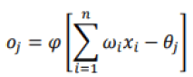
Where θj is a threshold specific to node j. The result obtained will depend on the activation function used φ. The output value can be used either as an input to a new layer of neurons or as a final result. The main types of this functions are:
1. Linear: φ is the identity function
2. Rectified linear unit: φ(x) = max (0, x)
3. Sigmoid:φ(x) = ex
4. Radical: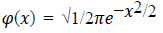
On R, after normalizing values we used the function "neuralnet" from the package that holds the same name, which used a sigmoid function as an activation function.
Support Vector Machines (SVMs)
Support vector machines (SVMs) are supervised learning algorithms, useful for both classification and regression problems. Support vector machines are algorithms that will classify the elements thanks to the hyperplane of optimal separation that we can call a "border". This is a separator that will maximize the margin, which refers to the distance between the classes. This algorithm is very useful in the case of large sets. In order to be able to use the "svm" function which allows the creation of the model, we installed the "e1071" package. We looked at different functions that the “kernel” can take, as well as the "cost" parameter which can be defined as the weight that penalizes the margin. Concerning the kernel, three functions were tested: the radial, linear and polynomial function. Nevertheless, it turns out that the radial function offered the best precision. Next, we retained a cost of 128 to optimize the model (Rasekhschaffe & Jones, 2019).
Evaluation of the Performance of the Machine Learning models
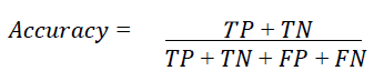
Once we use Machine Learning algorithms, it becomes important to measure their performance. Thus, there are several ways to achieve this. However, it should be noted that evaluating the performance of a classification algorithm is often more difficult than evaluating that of a regression algorithm. The first method concerns the confusion matrix which is a binary classifier. The idea behind this matrix is to make it easier to visualize performance and measure the percentage of misclassified individuals. The higher this percentage, the more we can question the efficiency and performance of the algorithm. On the rows of this matrix will be the predicted classes, while each column represents a real class.
On the main diagonal of this matrix are correctly classified cases (TN and TP), all other cells in the matrix contain misclassified examples. From this matrix, it is possible for us to calculate various measures. The best known is Accuracy and measures the number of correctly classified individuals out of the total number of individuals. It is therefore the sum of the elements of the diagonal of the matrix divided by the total of the matrix.
The matrix gives a lot of information, but sometimes we prefer a shorter measurement, called the Precision of a classifier which is measured as follows:
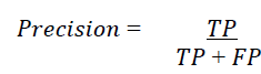
Where TP is the number of True Positives and FP the number of False Positives. The Precision will therefore be equal to 1, which is a perfect score, if the classifier predicts True Positives. This Precision is often used in combination with another measurement:
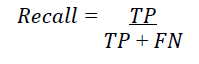
Where FN denotes the number of False Negatives. Recall measures the ratio of positive cases that were correctly detected by the algorithm. In some cases, it may be better to be successful in detecting unwanted cases than in detecting desired cases. In a situation where we are building a stock price prediction algorithm, it is better to maximize the Precision rather than the Recall because it is preferable to decrease the losses.
Precision and Recall are thus combined in the same measurement called F1 score, which is the harmonic mean of the two measurement tools. The harmonic mean, unlike the arithmetic mean, will give higher weight to low values. Therefore, a classifier’s F1 score will be high if both the Precision and Recall readings are high. The F1 score is calculated using the following formula (Basheer & Hajmeer, 2000).
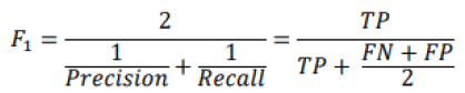
Unfortunately, increasing the Precision decreases the Recall, and vice versa which makes it difficult to get a high F1 score. This phenomenon is called the Precision / Recall compromise.
In the rest of this article, we will use the confusion matrices and Accuracy, which we will denote by the term "
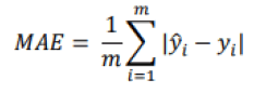
". For regression problems, there are also several evaluation methods. We will retain the three measures most cited in the literature: the Root Mean Square Error (RMSE), the Mean Absolute Error (MAE) and the R-squared (R2). The Root Mean Square Error (RMSE), applied to a system, will make it possible to define what is the level of error that the system will emit in its predictions. Larger errors are given greater weight. This measurement is expressed in the following mathematical form:
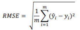
Where m is the number of individuals in the database, y is the predicted value of the dependent variable for individual i and yi is the observed, expected value for item i. A value of our RMSE of 0 would indicate that the regression model fits the data perfectly, so a small value is preferable. While this is the most widely used measurement tool for regression problems, there is another similar measurement, but more suitable to situations with many outliers. In this case, we prefer to apply the Mean Absolute Error (MAE) (Géron, 2019).
A final tool that is often used is the R-squared (coefficient of determination) or the adjusted R- squared. According to Miles (2014), these two measures are statistics derived from the general linear model analysis (regression, Anova). It represents the proportion of the variance explained by the predictor variables in the sample (R-squared) and a population estimator (adjusted R-squarred). It is therefore the proportion of the variance in the dependent variable that is predictable from the independent variables. In general, the closer the value is to 1, the better our model will be able to predict our dependent variable, even if in some situations a low R2 does not necessarily indicate a bad prediction. Indeed, certain fields of study, such as those on the human behavior, will always present unexplained variations. If the model has a high variance and the residuals are highly dispersed, our value for R2 will be small, but the regression line may still be the best prediction. R2 is expressed mathematically according to the following formula:
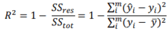
Where  is the mean of the values of the dependent variable. Another potential problem with R2 is that its value can increase with the addition of variables, without having a predictive quality. For this reason, we can use another metric that takes into account the number of independent variables and helps indicate whether a variable is "useless" or not: adjusted R- squared. As we add variables without predictive quality, the value of our adjusted R2 will be low and this can be seen in its mathematical formula where k is the number of independent variables:
Where n denotes the size of the sample. Its value will also be between 0 and 1 and will always be equal to or less than that of R2.
This step is essential for our Machine Learning models. In order to test our models, we used the "predict" function in R that will give a label for the new data and attempt to predict the signals with the best precision. In some cases, it was necessary to install an additional package, like the "caret" package for the Random Forest model. Once the predictions are done, we represented the results under confusion matrices and calculate the accuracy of our models to see if they were able to correctly predict the signals.
Calculation of the Returns and Performances
After obtaining the signals from our test data. Where, a signal of 1 corresponds to an increase in the price for the next day, and a signal of 0 to a decrease trend for the price the next day. It was possible to calculate the overall return of each model. In order to do this, we multiplied the returns for each period with the signal. That means that we take advantage of a return when the model predicts an increase in stock price. Next, we calculated the cumulative returns for each strategy. The cumulative return is calculated as follows:
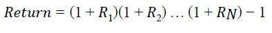
Where Ri is the return of the period i.
It is now interesting to measure the performance of the strategy. Regarding this, we used the Sharpe Ratio. This ratio, also called the reward / variability ratio that is a measure introduced in 1966 by William Sharpe that allows to estimate the performance of a portfolio to be measured by adjusting its risk. A high ratio is interpreted as a high return on investment in relation to the risk taken, and therefore it is a good investment. It is expressed mathematically as follows:
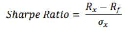
Where Rx is the portfolio return, Rf is the risk-free rate and σx is the standard deviation of the portfolio return, also called volatility. The risk-free rate refers to the interest rate that an investor can expect to earn on a risk-free investment. In this case, we have designated the Buy & Hold strategy applied to the S&P 500 Sariah as the risk-free investment. We considered the S&P 500 Sariah because the index covers a multiple number of sectors. As for volatility, it is calculated on the basis of daily returns. A positive Sharpe Ratio implies that the considered strategy is outperforming the Buy & Hold strategy. And a negative Sharpe Ratio therefore implies that the investment returns are too low for the risk considered.
Empirical Results
In order to verify which Machine Learning algorithm, perform better in the case of Islamic stock indexes. We calculated, first, our confusion matrixes in order to have a general idea on our predictions in Table 1.
| Table 1 Confusion Matrices |
|||||
|---|---|---|---|---|---|
| Indexes | MCSII | JKII | |||
| Models | Signals | High | Low | High | Low |
| CART | High | 278 | 227 | 0 | 0 |
| Low | 0 | 0 | 218 | 280 | |
| RF | High | 142 | 100 | 79 | 104 |
| Low | 136 | 127 | 139 | 176 | |
| ANN | High | 223 | 170 | 33 | 36 |
| Low | 55 | 57 | 185 | 244 | |
| SVM | High | 223 | 170 | 39 | 31 |
| Low | 55 | 57 | 179 | 249 | |
This measurement informs us of the number of elements that have been correctly classified. Next, it was possible for us to calculate the precision of our algorithm. This represents the ratio between correctly classified individuals and the total number of individuals in Table 2.
| Table 2 Precisions Of Ml Algorithms |
||
|---|---|---|
| Precision | ||
| MCSII | JKII | |
| CART | 55,05% | 56,22% |
| RF | 53,27% | 51,20% |
| ANN | 55,25% | 55,62% |
| SVM | 55,45% | 57,83% |
Finally, we calculated the Cumulative returns and the Sharpe Ratios which define the attractiveness of the strategy in Table 3 and Table 4.
| Table 3 Returns Of Ml Algorithms |
||
|---|---|---|
| Returns | ||
| MCSII | JKII | |
| CART | 8,63% | 54,22% |
| RF | 8,93% | 49,93% |
| ANN | 6,19% | 45,98% |
| SVM | 11,33% | 55,52% |
| Table 4 Sharpe Ratios Of Ml Algorithms |
||
|---|---|---|
| Sharpe Ratio | ||
| MCSII | JKII | |
| CART | -5,4 | -0,15 |
| RF | -7,76 | -0,42 |
| ANN | -10,55 | -0,48 |
| SVM | -6 | -0,55 |
First of all, by analyzing confusion matrices (table 1), especially for CART. We can see that the model only predicts increasing signals or decreasing signals. This is explained by the fact that the generated tree consists of one leaf, where the probability of a high signal is greater than that of a low signal or the opposite.
Regarding the precisions for the MCSII index predictions (table 2) over the studied period. We see from that the SVM model is the most accurate with an accuracy rate of 55.45%, followed by the ANN with 55.25% and then the CART tree with 55.05%. We also note that each of our models generally has a precision rate greater than 50% which question the low form of market efficiency. When it comes to returns, the SVM algorithm still comes first with a return of 11.33%, followed by RF with 8.93% and the CART model which comes in third with 8.63%.
The low returns are explained by the fact that some high signals were predicted as low signals, which includes some loss in returns. In order to complete this analysis, we will analyze the results of the Sharpe ratio which will allow us to assess the performance of our strategies and measure the level of return compared to the S&P 500 Sharia with the Buy & Hold strategy. We can see that our Sharpe ratios are all negative. This is mainly explained by the fact that the cumulative returns of each ML strategy are lower than the cumulative returns of the S&P 500 Sharia with the Buy & Hold strategy.
On the other hand, regarding the JKII index, we also see that all machine learning models also all offer a rate greater than 50%. At the top of the ranking, we have again the SVM, followed by the CART decision tree, and thirdly the ANN. Hence, we can say that this corresponds with the results of the first index.
In terms of cumulative returns, once again the SVM algorithm appears to perform better, which makes sense as accuracy rate and performance are closely related. If we now look at the Sharpe Ratios, these are all negative again. This is because none of the strategies can match the benchmark, namely the S&P 500 Sharia with the Buy & Hold strategy.
From these results, we can therefore say that investing in these indices during the period studied was a bad decision because the returns are too low compared to the risk considered. However, we can get a clear idea of which algorithm performs better and say that SVM outperforms other ML algorithms for both indices. Moreover, we can see that the majority of the predicted labels are correct and therefore our model allows us to question the weak efficiency theory of the markets which says that the historical price is directly reflected in the price, because it seems that it is possible to take advantage of arbitration opportunities.
Conclusion
As financial markets become super-connected entities where information exchange occurs rapidly. It is clear that many financial transactions are based on pre-defined rules. That makes the automation in finance very relevant in multiple cases. The machines are therefore required to perform their tasks by following the rules as quickly as possible. However, humans also base their decisions on their own instincts, rather than following a set of rules. Nevertheless, giving that a human being is not particularly perfect at making decisions based on facts, he can be subject to many biases, such as emotions, fears and hopes. In order to prevent any bias from skewing the results, the best solution is to rely on machines that offer a decision based on facts learned from concrete data showing the reality of the market as well as the laws of the market. Hence, the usefulness of using machine learning in prediction the performance of the market and rely on it as a powerful decision support tool.
In this context, this article aims to measure the performance of machine learning algorithms in the context of Islamic finance. In order to carry out this analysis, we carried out an empirical study, we were interested in two stock indices Morgan Stanley Capital International Islamic (MCSII) and the Jakarta Islamic Index (JKII) over a period of 10 years going from January 4, 2010 to January 2, 2020. We studied four Machine Learning models: A classification and regression tree (CART), a random forest model (RF), a neural network (ANN) and a support vector machine (SVM). We decided to compare these four algorithms using three independent variables in order to predict the price of the next day which take the value of 1 if it increases, or 0 if it falls. Next, we measured the cumulative return with these investment decisions. Thanks to the empirical results it was clear that the Machine Learning Algorithm (SVM) outperforms other algorithms in terms of both predictions and returns.