Keywords

Financial Institutions and Services; General; Banks, Depository Institutions, Micro Finance Institutions, Mortgages; Investment Banking, Government Policy, and Regulation.

JEL Code

G2, G20, G21, G24, G28.

Introduction

Research Question

In this article we have estimated the value of the Risk Weighted Asset-RWAs in European countries. Data from 30 European countries¹ were used except for the UK and Liechtenstein. The database used is that of the European Banking Authority-EBA.

The question of the riskiness of banks becomes increasingly important in both the European and global context due to a set of macroeconomic and international factors that significantly undermine the stability of the economy. The reference in this case is both to Covid19 and to the crisis induced by Russia's invasion of Ukraine with the rise in prices of raw materials globally. Furthermore, Western countries seem to face a further problem, namely the return of inflation, which seemed to have been forgotten for some time. Finally, the international banking system is involved in the tech-war between China and the USA which greatly stresses the markets due to the need to find investment methodologies in new technologies that can support levels of innovation and research and development capable of to make the West still competitive with the growing Asian powers. And again, the choice of major countries to invest in environmental sustainability increases the difficulty of the banking and financial system to find partners who are reliable and who can also comply with the guidelines chosen by the international community during the Paris agreements and the Glasgow Coop26.

In this context, the question of bank stability and the attempt to reduce the riskiness of bank assets becomes a priority to avoid that a further risk factor is added to the instability of a technological, international, and environmental macro-economic nature, namely the crisis. banking and finance. Controlling the level of banks' riskiness is therefore necessary to reduce the exposure of the entire European banking system to risks. In this sense, banking regulation and supervision is very important, which through the analysis of capital requirements and with the intervention in individual national banking systems can increase the degree of financial stability avoiding the manifestation of systemic risks and forms of contagion. amidst financial crises.

Certainly, the current scenario does not allow banks to find debtors who are reliable, and in fact the value of Non-Performing Loans-NPLs tends to grow both in the business sector and in the household credit sector. The result is therefore a dangerous growth in the spiral of risk which in the case of Europe also affects Germany, the leading country of the European economy.

However, growing inflation, the attempt by European and world governments to spend more to meet the consequences of covid19 and the energy crisis produced by the Russian attack on Ukraine, generate a request for credit with respect to which compliance with the European treaties turns out to be very complex. The European policy maker must therefore intervene to verify whether the construction of European banking, from the point of view of economic banking policies, can resist and in what way, with respect to the new threats offered by a change in the global order which on the one hand requires greater expenditure. public, and on the other hand, through inflation, tends to weaken the condition of creditors.

The article continues as follows: in the second paragraph a brief analysis of the essential literature is presented, in the third paragraph a 36-variable econometric model is presented, in the fourth paragraph the results of the clustering carried out with k-means algorithm are reported, in the fifth paragraph there are the predictions obtained through the comparison of performance between machine learning algorithms, the sixth paragraph concludes. Finally, the main statistical results are reported in the appendix.

Literature Review

The following section indicates some bibliographical references that are useful for framing the question of the role of WRAs in the context of the banking and financial stability of countries also considering the requirements of national and international banking regulation. (Ferri & Pesic, 2017) highlight the complex relationship existing between the growing value of WRAs, innovative bank accounting systems, and the purposes of prudential supervisory systems. Highlight the complex relationship existing between the growing value of WRAs, innovative bank accounting systems, and the purposes of prudential supervisory systems. (Juelsrud & Wold, 2020) Consider the strategies banks put in place to reduce the value of RWAs in Norway. Norwegian banks are raising capital requirements, reducing lending to businesses, and raising the interest rate. This choice while increasing the stability of the Norwegian banking system tends to be associated with a reduction in the value of employment created in the private sector. (Böhnke et al., 2022) highlight the complex relationship existing between the RWA value, the presence of Internal Rating Based-IRB and the banking regulation activity. The authors show that following the introduction of the IRB, a phenomenon was created whereby countries that had high levels of WRAs took on a strict prudential behavior, while countries that had low levels of WRAs increased the riskiness of their assets. The result is therefore a divergence with a role of banking supervision which tends to be more permissive or severe based on the riskiness of the countries. (Khan et al., 2017) show that banks with less liquidity also tend to be riskier as demonstrated by the growth in the value of WRAs. However, capital requirements tend to limit the operational capabilities of banks with low liquidity levels. It follows therefore that regulators can take action to prevent banks with reduced liquidity from increasing their exposure to risk.

(Abdul Wahab et al., 2017) find a positive and causal relationship between the value of the Capital Ratio and the value of the WRAs. The authors suggest that increasing capital requirements may reduce banks' ability to acquire risky assets. (Esposito et al., 2019) propose a measure of the RWAs to consider the role of the environment in the credit allocation choices of banks with an impact also in terms of banking regulation and supervision policies. (Santos, et al., 2020) analyze the reasons that lead to an increasing variability in the value of RWAs. The authors compare an indicator of the market's RWAs with the RWAs indices produced by the same banks. The result shows that the value of RWAs attributed by external evaluators tends to be higher than the value of RWA communicated autonomously by the banks. This difference is since while on the one hand external market observers attribute an additional value to RWA to consider the value of the banks' opaque operations, on the other hand banks tend to omit information relating to riskiness.

(Nkwaira & Kruger, 2018) propose an alternative way to distribute banks' risks using insurance contracts while respecting the regulatory requirements of Basilea III. (Strickland, 2017) shows alternative methods to calculate RWA in the light of new technologies. (JIN, 2019) finds that banks adjust RWA in response to changes in capitalization.

(Brei et al., 2020) consider the impact of low interest rates on the intermediation activities of 113 banks over the period 1994-2015. The authors verify an increase in the value of the margin deriving from trading activities with a reduction in the RWA. (Nguyen, 2019) derive the Risk Weighted Function to calculate RWA.

The Econometric Model

We found that the RWA volume is negatively associated with:

• Distribution of NFC loans and advances by NACE code (other than trading exposures) - B Mining and quarrying: the relationship represents the complex of loans and advances that banks give to non-financial companies operating in the mining and quarrying sector. There is therefore a negative relationship between the value of risk weighted assets and the value of the debt exposure to non-financial companies operating in the mining sector.
• Distribution of NFC loans and advances by NACE code (other than trading exposures) - O Public administration and defence, compulsory social security: represents the investment in terms of loans and advances that is made in the context of non-financial corporations operating in the public administration, defense and compulsory social security sectors.
• Distribution of NFC loans and advances by NACE code (other than trading exposures) - K Financial and insurance activities represents the amount of loans and advances that are provided to non-financial companies operating in the financial and insurance sector. There is therefore a negative relationship between the value of risk-adjusted assets and the value of bank investments in NFCs operating in the finance and insurance sector. • Components of RoE: Staff expenses / equity: It is the relationship between personnel expenses and the value of equity. There is a negative relationship between the value of risk-adjusted assets and the value of risk-adjusted personnel expenses. This value is due to a dual combined effect, namely that of the numerator consisting of personnel expenses and that of the denominator or equity.
• Loans and advances at amortised cost: NPL ratio – NFCs: is a variable that considers the relationship between Non Performing Loans and the gross book values ??for companies that are NFC.
• Loans and advances at amortised cost: NPL ratio – HHs:  it is a variable that considers the relationship between NPLs and gross value with reference to the loans that are offered to households. The growth of NPLs vis-à-vis households is associated with a negative value of RWAs. This relationship might seem counterfactual and yet it demonstrates that the credit that banks offer to households does not generate significant losses for the bank as it could happen because of financial investments.
• Distribution of NFC loans and advance for NFC in accommodation and food service activities: is a variable that considers the value of the loans and advances made to companies operating in the hotel and food sectors. These are businesses that are NFC. The investment in this sector of economic activity reduces the value of the RWAs creating advantages of financial stability in the economies of the countries considered.
• Liabilities composition - Customer deposits from HHs: is a ratio between the value of household deposits and the value of total liabilities. There is a negative relationship between the value of this ratio and the value of RWAs. Since RWAs tend to grow in financial crises, it follows that the credit that banks offer to households increases the financial stability of national banking systems.
• Components of RoE: Other operating income / equity: is a ratio consisting of [Total net operating income - net interest income - Fee & commission income - net trading income (A)] / [Equity (B)]. This ratio is negatively associated with the value of RWAs. Since the growth of RWAs manifests the growth of risks in the national and international banking system, it follows that the value of the risks is reduced when banks prefer traditional intermediation margins over those deriving from financial investments.
• Composition of own funds (Tier 1 capital) - Accumulated other comprehensive income: is a ratio considered as follows: [Accumulated other comprehensive income (A)] / [Tier 1 capital volume (B)]. The growth in the value of the accumulated other inclusive income compared to the value of the Tier 1 capital volume is negatively associated with the value of RWAs. It therefore follows that if even potential income increases, net of potential losses, the value of RWAs tends to decrease with a significant advantage for the safety of the national banking system.
• Sovereign exposure - Total gross carrying amount by maturity: 5Y - 10Y: represents the total gross book value of the assets. This value is negatively associated with the RWAs value. It follows that an increase in the total gross book value of assets improves the condition of the bank from the point of view of riskiness.
• Non-performing loans and advances at amortised cost – NFCs: considers the gross carrying amount of amortized impaired loans to non-financial corporations. This variable is negatively associated with the value of RWAs with an improvement in the risk conditions of the banking systems.
• Loans and advances at amortised cost - NFCs, of which SMEs: represents the gross value of loans to small and medium-sized enterprises that are not financial companies.
• Loans and advances at amortised cost - HHs, of which mortgages: is the gross book value of the loans that have been made to households with attention to mortgages secured by real estate.
• Sovereign exposure - Total carrying amount (net of short positions): Debt exposure to governments net of short positions.

We also find that the level of RWA volume is positively associated to:

It is generally possible to verify that the value of RWAs tends to rise in times of financial crises shows in Table 1. Therefore, the analysis conducted may be useful to understand which types of transactions are most compatible with a reduction in the value of RWAs in European banking systems. In this sense, there are certainly sectors that present a particular risk in terms of RWAs growth and among these are: Real Estate, Administrative and Support Service Activities, Other Services, Construction, Human Health Services and Social Work Activities and Education. On the contrary, there are sectors that are negatively associated with the value of RWAs and which can therefore be considered as tools that can reduce the risk value of countries, namely: Mining and quarrying, Public administration and defense, compulsory social security, Financial and insurance, accommodation and food service.

Table 1 Different Variable Financial Assest
N	Variable	Explanations
1	Total fair valued financial assets	Total financial instruments on the asset side
2	Sovereign exposure Total gross carrying amount	Total gross carrying amount
3	Contingent liabilities loan commitments volume	Gross carrying amount
4	Loans and advances at amortised cost HH:	Households (A) / Total Loans and advances with non-expired EBA-compliant moratoria (B)
5	Loans and advances at amortised cost NFCs	NFCs (A) Total Loans and advances with non-expired EBA-complant moratoria (B)
6	Composition of own funds (Tier / capital) Own funds (Tier / capital) volume
7	Sovereign exposure Total carrying amount (net of short positions), of which: Fair value through OCI	Sovereign exposure treated as Fair value through OCI (A) Sum of the sovereign exposure values at fair value through P&L OCI and amortised cost (B)
8	Non-performing loans and advances at amortized cost HHs	Gross carrying amount of non-performing loans at amortised costs to Households
9	Non-performing loans and advances at amortised cost NFCs, of which CRE	Gross carrying amount of non-performing loans at amortised costs to NFCs of which Loans collateralised by commercial immovable property
10	Liabilities composition Customer deposits from NFCs	Deposits from NFCs (A) Total liabilities (B)
11	Composition of own funds (Tier / capital) Capital instruments eligible as CETI Capital	Capital instruments eligible as CET1 Capital (A) Tier 1 capital volume (B)
12	Non-performing loans and advances at amortised cost: coverage ratio HH:
13	NPL ratios of NFC loans and advances by NACE code (other than trading exposures) L Real estate activities	NFCs loans and advances - L Real estate activities (A) Total gross carrying amount Loans and advances (B)
14	NPL ratios of NFC loans and advances by NACE code (other than trading exposures) N Administrative and support service activities	NFCs loans and advances N Administrative and support service activities (A) Total gross carrying amount Loans and advances (B)
15	Contingent liabilities Share of loan commitments to HH:	Loan commitments to HHs (A) Total loan commitments given (B)
16	NPL ratios of NFC loans and advances by NACE code (other than trading exposures) $ Other services	NFCs loans and advances . $ Other services (A) Total gross carrying amount Loans and advances (B
17	NPL ratios of NFC loans and advances by NACE code (other than trading exposures) F Construction	NFCs loans and advances F Construction Non-performing (A) Loans and advances (B)
18	Distribution of NFC loans and advances by NACE code (other than trading exposures) F Construction	Exposures to NACE F (Construction) (A) Total exposures to non-financial corporations (B)
19	Distribution of NFC loans and advances by NACE code (other than trading exposures) 0 Human health services and social work activities	NFCs loans and advances Q Human health services and social work activities (A) / Total gross carrying amount Loans and advances (B)
20	Components of RoE: Net fee & commission income / equity	Fee & commission income - Fee & commission expense (A) / Equity (B
21	Distribution of NFC loans and advances by NACE code (other than trading exposures) P Education	INFCs loans and advances P Education (A) Total gross carrying amount Loans and advances (B)

Clusterization

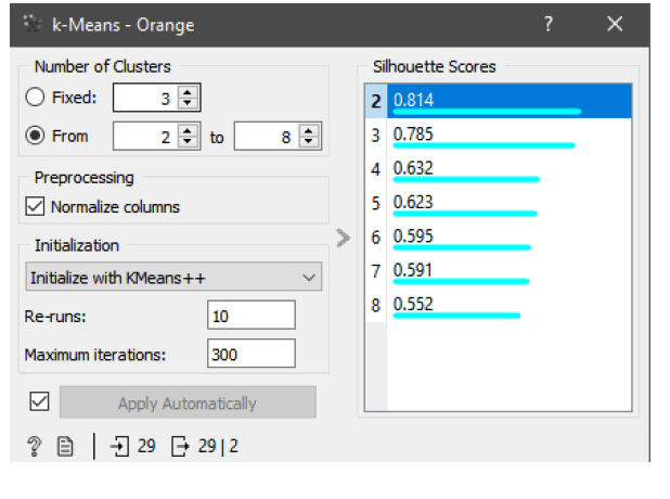
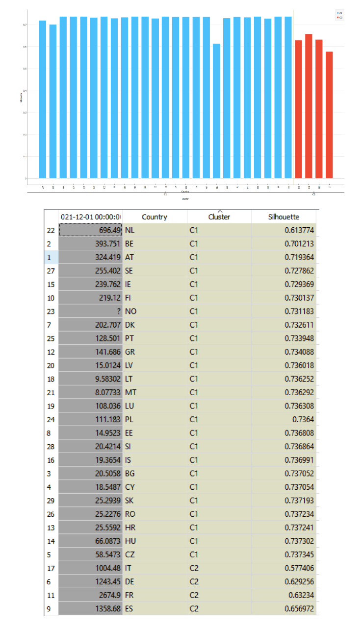
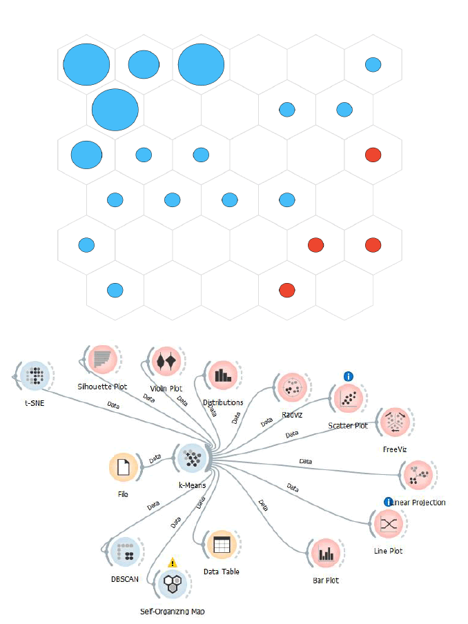
Below is a representation of a clustering analysis carried out using the k-means algorithm. The criterion of maximizing the Silhouette coefficient was used to choose the number of clusters. The Silhouette coefficient varies between -1 and 1. In the analyzed case, eight different types of clustering were tested, and the result is that the number of clusters associated with the highest silhouette coefficient is equal to two.

The countries that are part of each cluster are indicated below, that is:

• Cluster 1: Netherlands with an RWA value of 696.49, Belgium with an RWA value of 393.751, Austria with a value of 324.41, Sweden with a value of 255.402, Ireland with an amount equal to 23.76, Finland with an amount equal to 219.12, Norway with an amount equal to 117.52, Denmark with an amount equal to 202.707, Portugal with an amount equal to 128.51, Greece with a value equal to 141.686, Latvia with an amount of 9.58, Malta with an amount of 8.07, Luxembourg with an amount of 108.036, Poland with an amount of 111.183, Slovenia with an amount of 20.42, Iceland with an amount of 19.36, Bulgaria with an amount equal to 20.50,

• Cluster 2: Italy with a value of RWA equal to 1004.48, Germany with a value equal to 1243.45, France with a value equal to 2674.9, Spain with an amount equal to 1358.68.

If we take into consideration the median value for each single cluster, we can see that the median value of the RWAs for the countries of cluster 1-C1 is equal to 66.0873 while the corresponding value for the countries of cluster 2-C2 is equal to 1301.065. It follows therefore that C2> C1. As we can see, there is therefore a significant and substantial difference within the European countries between the nations that are part of cluster 1 and the nations that are part of cluster 2. Specifically, the nations of cluster 2 have much higher levels of RWAs than to those of cluster 1 countries. In percentage terms, the value of cluster 2 countries has a median value of RWA equal to approximately 1868% compared to cluster 1. It therefore follows that there is a rift between the countries of cluster 2 in a condition of structural fragility compared to the countries of cluster 1. If we analyze the countries of cluster 2 among these there are both Spain, Italy and France which are notoriously considered risky countries in terms of assets. However, in cluster 2 there is also Germany which generally tends to have a much higher level of security and financial stability than that of France, Spain, and Italy. It follows therefore that Germany has also entered the ranks of high-risk countries from a banking and financial point of view and this condition is certainly an element of risk and instability for the whole of the European Union shows in Figure 1.

Furthermore, if we take the cluster 1 countries that show a higher level of RWAs, we can verify that these include Netherlands, Belgium, Austria, Sweden, and Ireland. These are countries that have very close commercial and economic relations with the countries of Cluster 2 and especially with Germany in the case of Netherlands, Belgium, and Austria. The result is therefore a scenario in which there is a Central-Southern area of Europe essentially made up of countries that have a dangerously growing and converging upward level of RWAs. The element that can certainly cause particular concern is Germany. However, it is likely that Germany has increased its value of RWAs following the various crises that have affected European countries and which have prompted Germany to also take on risky investments in other countries.

Furthermore, if we take the value of the average variation in the value of RWAs between the countries of cluster 1 and the countries of cluster 2, it appears that on average in the period analyzed the value of C1 has grown by an amount equal to 1.66 units in absolute value and by 1.29% while the corresponding value for the countries of cluster 2-C2 increased by 25.20 units equal to 1.63%. That is, even in a dynamic comparison between C1 countries and C2 countries, the value of the growth rate of RWAs tends to grow more for the C2 countries than for the C1 countries.

Machine Learning and Predictions

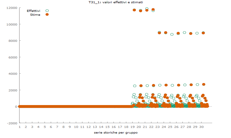
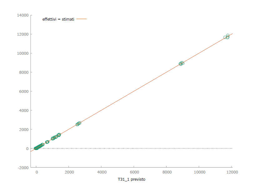
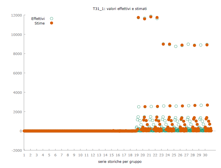
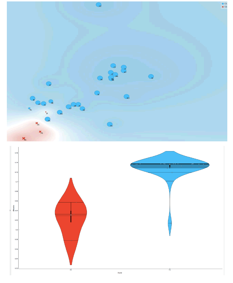
A comparison was made below between eight different machine learning algorithms to predict the future value of RWAs in the countries considered between the first quarter of 2019 and the fourth quarter of 2021. The algorithms were trained with 70% of the available data while the remaining 30% of the data was used for the actual prediction. The choice of the algorithm with the greatest predictive capacity took place through the ability to maximize the R-framework and minimize statistical errors, that is: mean absolute error, mean squared error, and root mean squared error shows in Figure 2.

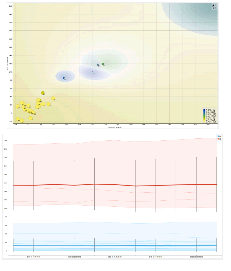
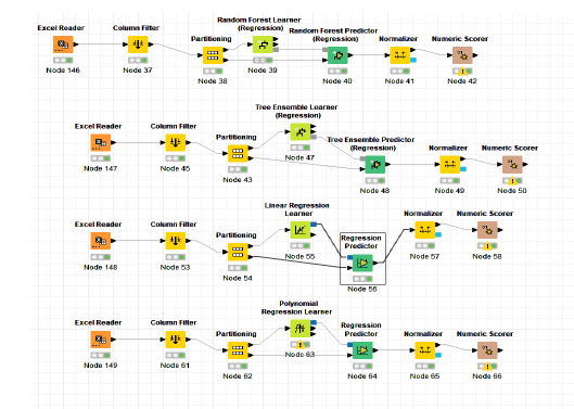
A ranking for each indicator was assigned to each algorithm and these rankings were then added together in the determination of a ranking of the algorithms by performative capacity in terms of prediction efficiency based on machine learning. The following ordering of the algorithms is therefore derived, that is:

1. Linear Regression with a payoff value of 4;
2. Tree Ensemble Regression with a payoff value of 8;
3. Random Forest Regression with a payoff value of 12;
4. Probabilistic Neural Network-PNN with a payoff value of 16;
5. Gradient Boosted Tree Regression with a payoff value of 20;
6. Simple Regression Tree with a payoff value of 24;
7. ANN-Artificial Neural Network with a payoff value of 28;
8. Polynomial Regression with a payoff value of 32.

It follows that the best performer algorithm for predicting the RWAs value among the countries considered is linear regression.

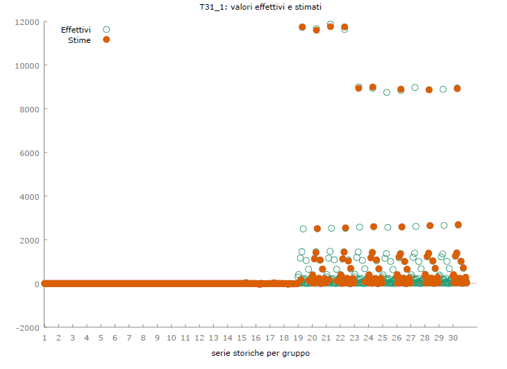
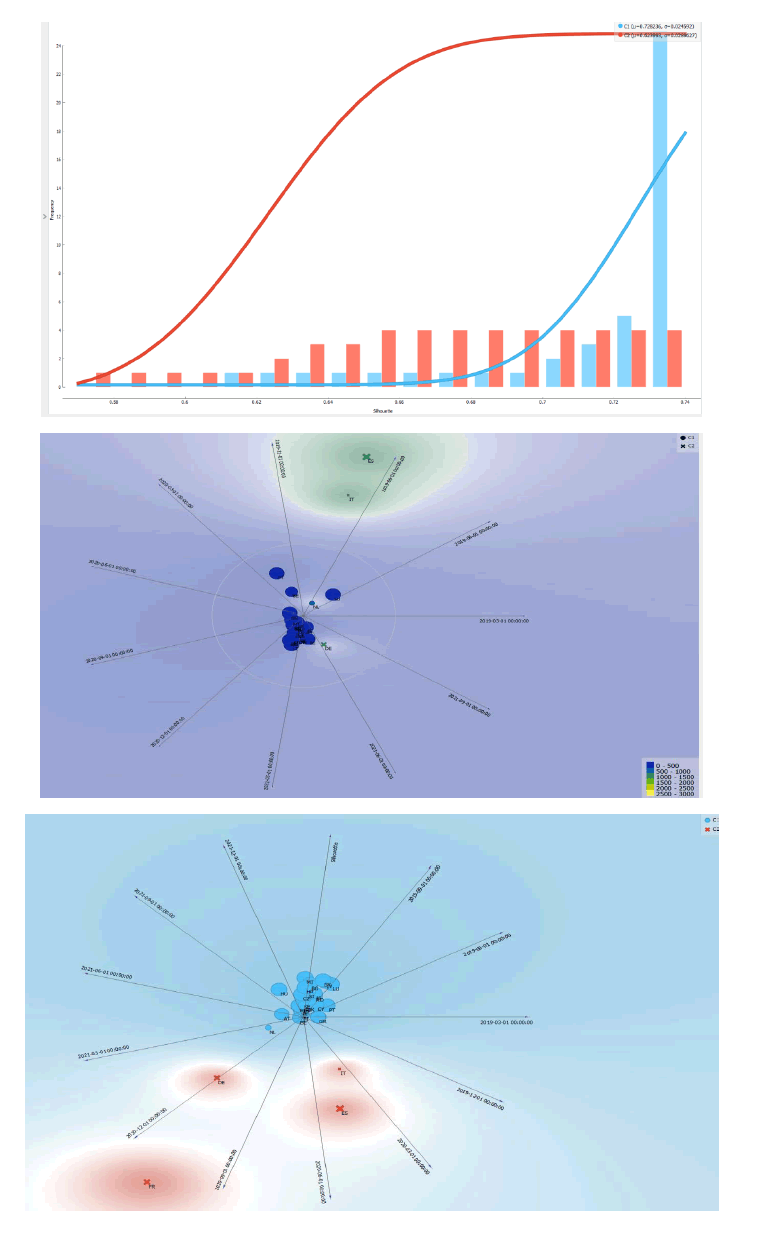
In this article we have used data from the European Banking Authority to estimate the determinants of WRAs in European countries. The data were analyzed using three methods, namely: a panel econometric model with 36 variables, a cluster analysis carried out with the k-means algorithm and the use of eight different machine learning algorithms for the prediction of the value of WRAs for the countries considered. The analysis shows that there are certainly investment sectors that increase the risk of banks, among which certainly there are the construction sector and the real estate sector, while other sectors are less risky such as the mining sector. minerals. Clustering also shows that in Europe there are two clusters of which one is virtuous and is made up of the countries of Northern and Eastern Europe and the other tends to be very risk-oriented and is made up of France, Italy, Spain, and Germany. The fact that Germany has a high level of banking risk can represent an element of financial instability for the entire European Union. Finally, the prediction shows that the level of RWAs will grow by 1.5% for the countries analyzed shows in Figure 3.

The expected rise in the level of RWAs should alarm the European policy maker. In fact, the mix of Covid19, the Russo-Ukraine war, inflation, low economic productivity, growth in energy prices, increase in public spending, creates a difficult condition for the banking sector against which it is necessary to intervene both in the revision of the treaties and also in the construction of new European institutions that are able to absorb the growing NPLs and distribute the risk more evenly among the EU countries.

Endnotes

¹ Countries are AT, BE, BG, CY, CZ, DE, DK, EE, ES, EU, FI, FR, GR, HR, HU, IE, IS, IT, LT, LU, IE, IS, IT, LT, LU, LV, MT, NL, NO, PL, PT, RO, SE, SI, SK.

References

Abdul Wahab, H., Saiti, B., Rosly, S. A. & Masih, A.M.M. (2017). Risk-taking behavior and capital adequacy in a mixed banking system: new evidence from Malaysia using dynamic OLS and two-step dynamic system GMM estimators. Emerging Markets Finance and Trade, 53(1), 180-198.

Indexed at, Google Scholar, Cross Ref

Böhnke, V., Ongena, S.R.G., Paraschiv, F., & Reite, E.J. (2022). Back to the roots of internal credit risk models: Why Do Banks’ Risk-weighted asset levels converge over time? Swiss Finance Institute Research Paper.

Brei, M., Borio, C., & Gambacorta, L. (2020). Bank intermediation activity in a low?interest?rate environment. Economic Notes, 2(e12164), 49.

Indexed at, Google Scholar, Cross Ref

Santos, E.B., Esho, N., Farag, M., & Zuin, C. (2020). Variability in risk-weighted assets: What does the market think. BIS.

Esposito, L., Mastromatteo, G., & Molocchi, A. (2019). Environment–risk-weighted assets: Allowing banking supervision and green economy to meet for good. Journal of Sustainable Finance & Investment, 9(1), 68-86.

Indexed at, Google Scholar, Cross Ref

Ferri, G., & Pesic, V. (2017). Bank regulatory arbitrage via risk weighted assets dispersion. Journal of Financial Stability, 33, 331-345.

Indexed at, Google Scholar, Cross Ref

JIN, O.L. (2019). The effect of bank capitalization on lending: Evidence from banks in Asia. Thesis-University Of Singapore.

Juelsrud, R.E., & Wold, E.G. (2020). Risk-weighted capital requirements and portfolio rebalancing. Journal of Financial Intermediation, 41(100806).

Khan, M.S., Harald, S., & Eliza, W. (2017). Funding liquidity and bank risk taking. Journal of Banking & Finance, 82, 203-216.

Indexed at, Google Scholar, Cross Ref

Nguyen, V.P. (2019). An attempt to derive the Risk Weight Function for the bank. University Library of Munich, Germany, 100631.

Nkwaira, C., & Kruger, J.W. (2018). Using risk-weighted assets to generate risk-weighted fees to counter the effects of basel iii on revenue generation. Journal of Finance, 6(2), 48-54.

Google Scholar

Strickland, O.J. (2017). Seeking to have banks sing to the same tune: The Basel committee addresses credit risk-weighted assets. University of Miami Business Law Review, 26(95).

Indexed at, Google Scholar

Appendix

Regressions

Modello 109: WLS, usando 724 osservazioni Incluse 27 unità cross section Variabile dipendente: T31_1 Pesi basati sulle varianze degli errori per unità
	Coefficiente	Errore Std.	rapporto t	p-value
const	2,62518e-05	0,00439125	0,005978	0,9952
T04_6	-150,979	10,9774	-13,75	<0,0001	***
T04_7	25,9787	15,1600	1,714	0,0870	*
T05_2	0,372489	0,0384916	9,677	<0,0001	***
T05_3	123,298	11,6984	10,54	<0,0001	***
T14_0	0,000856871	0,000426087	2,011	0,0447	**
T15_1	0,222624	0,0539134	4,129	<0,0001	***
T15_4	-0,237767	0,0569095	-4,178	<0,0001	***
T15_7	6,23588	2,94417	2,118	0,0345	**
T16_4	-10,1456	4,68384	-2,166	0,0306	**
T20_2	0,524952	0,0314039	16,72	<0,0001	***
T20_3	-0,420101	0,0274099	-15,33	<0,0001	***
T20_4	0,556490	0,0210369	26,45	<0,0001	***
T20_5	-1,03392	0,0263233	-39,28	<0,0001	***
T21_2	6,79421	0,325730	20,86	<0,0001	***
T21_4	-6,79405	0,642993	-10,57	<0,0001	***
T21_6	13,7203	1,49844	9,156	<0,0001	***
T22_2	-521,976	45,3583	-11,51	<0,0001	***
T22_4	-631,652	85,0932	-7,423	<0,0001	***
T23_2	38,7002	7,94597	4,870	<0,0001	***
T24_2	-1354,14	140,126	-9,664	<0,0001	***
T24_6	400,194	36,4667	10,97	<0,0001	***
T24_9	-347,154	51,3209	-6,764	<0,0001	***
T25_1	-765,732	58,4673	-13,10	<0,0001	***
T25_5	-1352,73	428,851	-3,154	0,0017	***
T25_6	5368,09	541,404	9,915	<0,0001	***
T25_7	718,210	89,2312	8,049	<0,0001	***
T26_6	260,152	28,1986	9,226	<0,0001	***
T27_2	93,0026	37,5927	2,474	0,0136	**
T27_4	122,614	25,9522	4,725	<0,0001	***
T27_9	173,495	20,4037	8,503	<0,0001	***
T28_3	777,478	66,9691	11,61	<0,0001	***
T28_5	-137,074	44,3147	-3,093	0,0021	***
T29_1	-736,919	83,3333	-8,843	<0,0001	***
T30_1	2,98629	0,110843	26,94	<0,0001	***
T30_2	27,7293	3,79870	7,300	<0,0001	***
T30_4	-109,291	17,0083	-6,426	<0,0001	***

Statistiche basate sui dati ponderati:
Somma quadr. residui	195,5848	E.S. della regressione	0,533567
R-quadro	0,999912	R-quadro corretto	0,999908
F(36, 687)	217433,9	P-value(F)	0,000000
Log-verosimiglianza	-553,5269	Criterio di Akaike	1181,054
Criterio di Schwarz	1350,691	Hannan-Quinn	1246,526

Statistiche basate sui dati originali:
Media var. dipendente	205,2978		SQM var. dipendente	1170,524
Somma quadr. residui	123080,0		E.S. della regressione	13,38491

Modello 110: Pooled OLS, usando 724 osservazioni Incluse 27 unità cross section Lunghezza serie storiche: minimo 2, massimo 30 Variabile dipendente: T31_1
	Coefficiente	Errore Std.	Rapporto t	p-value
const	0,168669	0,529903	0,3183	0,7504
T04_6	-159,572	13,2638	-12,03	<0,0001	***
T04_7	34,7485	19,1322	1,816	0,0698	*
T05_2	0,478211	0,0415995	11,50	<0,0001	***
T05_3	144,748	14,9839	9,660	<0,0001	***
T14_0	0,00649812	0,000904746	7,182	<0,0001	***
T15_1	0,402321	0,0917264	4,386	<0,0001	***
T15_4	-0,446291	0,0972225	-4,590	<0,0001	***
T15_7	15,0679	5,24483	2,873	0,0042	***
T16_4	-27,3710	8,69372	-3,148	0,0017	***
T20_2	0,437881	0,0359510	12,18	<0,0001	***
T20_3	-0,302772	0,0308001	-9,830	<0,0001	***
T20_4	0,508623	0,0211708	24,02	<0,0001	***
T20_5	-0,967576	0,0314684	-30,75	<0,0001	***
T21_2	6,67985	0,392569	17,02	<0,0001	***
T21_4	-4,07505	0,712413	-5,720	<0,0001	***
T21_6	8,03132	1,65099	4,865	<0,0001	***
T22_2	-417,916	55,0539	-7,591	<0,0001	***
T22_4	-799,994	102,589	-7,798	<0,0001	***
T23_2	51,2914	9,70600	5,285	<0,0001	***
T24_2	-1668,11	163,388	-10,21	<0,0001	***
T24_6	498,610	46,0669	10,82	<0,0001	***
T24_9	-451,246	64,7516	-6,969	<0,0001	***
T25_1	-742,853	66,5977	-11,15	<0,0001	***
T25_5	-1509,78	475,767	-3,173	0,0016	***
T25_6	5919,37	649,344	9,116	<0,0001	***
T25_7	761,900	109,213	6,976	<0,0001	***
T26_6	261,180	31,8690	8,195	<0,0001	***
T27_2	120,130	46,3795	2,590	0,0098	***
T27_4	150,399	31,6864	4,746	<0,0001	***
T27_9	181,355	25,3460	7,155	<0,0001	***
T28_3	769,591	79,1361	9,725	<0,0001	***
T28_5	-131,831	59,2890	-2,224	0,0265	**
T29_1	-830,630	98,9909	-8,391	<0,0001	***
T30_1	2,68493	0,129694	20,70	<0,0001	***
T30_2	34,0004	4,60227	7,388	<0,0001	***
T30_4	-135,686	21,4044	-6,339	<0,0001	***

Media var. dipendente	205,2978		SQM var. dipendente	1170,524
Somma quadr. residui	95103,87		E.S. della regressione	11,76578
R-quadro	0,999904		R-quadro corretto	0,999899
F(36, 687)	198752,7		P-value(F)	0,000000
Log-verosimiglianza	-2793,123		Criterio di Akaike	5660,247
Criterio di Schwarz	5829,884		Hannan-Quinn	5725,719
rho	0,024946		Durbin-Watson	1,738821

Modello 111: Effetti fissi, usando 724 osservazioni Incluse 27 unità cross section Lunghezza serie storiche: minimo 2, massimo 30 Variabile dipendente: T31_1
	Coefficiente	Errore Std.	rapporto t	p-value
const	0,214346	2,50137	0,08569	0,9317
T04_6	-145,638	12,6330	-11,53	<0,0001	***
T04_7	39,9668	21,0601	1,898	0,0582	*
T05_2	0,543400	0,0437317	12,43	<0,0001	***
T05_3	138,694	14,6884	9,442	<0,0001	***
T14_0	0,00536671	0,000892920	6,010	<0,0001	***
T15_1	0,529393	0,0867660	6,101	<0,0001	***
T15_4	-0,576875	0,0918646	-6,280	<0,0001	***
T15_7	15,4097	5,04897	3,052	0,0024	***
T16_4	-42,5524	10,0247	-4,245	<0,0001	***
T20_2	0,492449	0,0366131	13,45	<0,0001	***
T20_3	-0,331629	0,0308271	-10,76	<0,0001	***
T20_4	0,469104	0,0231082	20,30	<0,0001	***
T20_5	-0,953439	0,0308889	-30,87	<0,0001	***
T21_2	6,28498	0,369166	17,02	<0,0001	***
T21_4	-4,80173	0,700131	-6,858	<0,0001	***
T21_6	9,95318	1,63368	6,092	<0,0001	***
T22_2	-357,491	51,7604	-6,907	<0,0001	***
T22_4	-788,913	96,9264	-8,139	<0,0001	***
T23_2	51,9815	9,30538	5,586	<0,0001	***
T24_2	-2050,51	162,887	-12,59	<0,0001	***
T24_6	534,096	44,0632	12,12	<0,0001	***
T24_9	-433,784	62,2406	-6,969	<0,0001	***
T25_1	-636,110	67,5865	-9,412	<0,0001	***
T25_5	-1908,01	468,956	-4,069	<0,0001	***
T25_6	5098,36	630,071	8,092	<0,0001	***
T25_7	929,385	111,697	8,321	<0,0001	***
T26_6	179,705	31,4823	5,708	<0,0001	***
T27_2	157,428	44,4204	3,544	0,0004	***
T27_4	172,139	29,8536	5,766	<0,0001	***
T27_9	166,674	25,2341	6,605	<0,0001	***
T28_3	808,088	75,1046	10,76	<0,0001	***
T28_5	-172,341	55,4817	-3,106	0,0020	***
T29_1	-843,272	107,493	-7,845	<0,0001	***
T30_1	2,54929	0,132618	19,22	<0,0001	***
T30_2	35,9774	4,37690	8,220	<0,0001	***
T30_4	-153,810	20,1927	-7,617	<0,0001	***

Media var. dipendente	205,2978		SQM var. dipendente	1170,524
Somma quadr. residui	77818,56		E.S. della regressione	10,85028
R-quadro LSDV	0,999921		R-quadro intra-gruppi	0,999904
LSDV F(62, 661)	135703,6		P-value(F)	0,000000
Log-verosimiglianza	-2720,510		Criterio di Akaike	5567,020
Criterio di Schwarz	5855,862		Hannan-Quinn	5678,500
rho	-0,003996		Durbin-Watson	1,843883

Test congiunto sui regressori -
 Statistica test: F(36, 661) = 190341
 con p-value = P(F(36, 661) > 190341) = 0 Test per la differenza delle intercette di gruppo -
Ipotesi nulla: i gruppi hanno un'intercetta comune
Statistica test: F(26, 661) = 5,64706
con p-value = P(F(26, 661) > 5,64706) = 1,11963e-016

Modello 112: Effetti casuali (GLS), usando 724 osservazioni Con trasformazione di Nerlove Incluse 27 unità cross section Lunghezza serie storiche: minimo 2, massimo 30 Variabile dipendente: T31_1
	Coefficiente	Errore Std.	z	p-value
const	1,67737	3,76129	0,4460	0,6556
T04_6	-145,385	12,3720	-11,75	<0,0001	***
T04_7	45,5550	18,8988	2,410	0,0159	**
T05_2	0,524068	0,0417800	12,54	<0,0001	***
T05_3	142,332	14,1848	10,03	<0,0001	***
T14_0	0,00574235	0,000880587	6,521	<0,0001	***
T15_1	0,500580	0,0857463	5,838	<0,0001	***
T15_4	-0,547602	0,0908128	-6,030	<0,0001	***
T15_7	13,8337	4,95532	2,792	0,0052	***
T16_4	-43,7852	9,87455	-4,434	<0,0001	***
T20_2	0,478913	0,0350646	13,66	<0,0001	***
T20_3	-0,325883	0,0298699	-10,91	<0,0001	***
T20_4	0,479909	0,0221508	21,67	<0,0001	***
T20_5	-0,954517	0,0304001	-31,40	<0,0001	***
T21_2	6,34708	0,366204	17,33	<0,0001	***
T21_4	-4,71706	0,685194	-6,884	<0,0001	***
T21_6	9,71256	1,59731	6,081	<0,0001	***
T22_2	-366,671	51,2901	-7,149	<0,0001	***
T22_4	-786,724	95,7557	-8,216	<0,0001	***
T23_2	54,0909	9,21150	5,872	<0,0001	***
T24_2	-1952,92	158,544	-12,32	<0,0001	***
T24_6	535,405	43,2262	12,39	<0,0001	***
T24_9	-442,417	61,0437	-7,248	<0,0001	***
T25_1	-628,220	64,3754	-9,759	<0,0001	***
T25_5	-1856,72	457,784	-4,056	<0,0001	***
T25_6	5306,05	610,961	8,685	<0,0001	***
T25_7	903,445	106,281	8,501	<0,0001	***
T26_6	186,222	31,1599	5,976	<0,0001	***
T27_2	156,677	44,0416	3,557	0,0004	***
T27_4	172,823	29,6466	5,829	<0,0001	***
T27_9	163,278	24,1152	6,771	<0,0001	***
T28_3	806,288	74,3448	10,85	<0,0001	***
T28_5	-163,962	54,8705	-2,988	0,0028	***
T29_1	-824,910	98,6179	-8,365	<0,0001	***
T30_1	2,59669	0,126623	20,51	<0,0001	***
T30_2	36,1746	4,30615	8,401	<0,0001	***
T30_4	-151,218	19,9322	-7,587	<0,0001	***

Media var. dipendente	205,2978		SQM var. dipendente	1170,524
Somma quadr. residui	116335,1		E.S. della regressione	13,00353
Log-verosimiglianza	-2866,068		Criterio di Akaike	5806,137
Criterio di Schwarz	5975,774		Hannan-Quinn	5871,609
rho	-0,003996		Durbin-Watson	1,843883

Varianza 'between' = 261,593
Varianza 'within' = 107,484
theta medio = 0,855389
Test congiunto sui regressori -
Statistica test asintotica: Chi-quadro(36)=7,0787e+006
con p-value = 0 Test Breusch-Pagan -
 Ipotesi nulla: varianza dell'errore specifico all'unità = 0
 Statistica test asintotica: Chi-quadro(1) = 2,78663
 con p-value = 0,0950539 Test di Hausman -  Ipotesi nulla: le stime GLS sono consistenti
Statistica test asintotica: Chi-quadro(13) = 19,3027
con p-value = 0,114014

Clusterization

Neural Networks and Machine Learning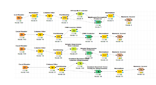

Prediction With Linear Regression
Countries	2021	Prediction	Var Ass	Var Per
CY	18,540	20,587	2,047	11,041
HR	25,550	27,406	1,856	7,264
HU	66,087	70,778	4,691	7,098
IS	19,365	20,158	0,793	4,095
LU	108,036	105,088	-2,948	-2,729
MT	8,077	9,722	1,645	20,366
NL	696,490	705,130	8,640	1,241
PL	111,183	110,824	-0,359	-0,323
SK	25,294	25,108	-0,186	-0,735
Mean	119,847	121,645	1,798	1,500

Received: 04-Nov-2022, Manuscript No. AEJ-22-12798; Editor assigned: 05-Nov-2022, PreQC No. AEJ-22-12798(PQ); Reviewed: 16-Nov-2022, QC No. AEJ-22-12798; Revised: 22-Nov-2022, Manuscript No. AEJ-22-12798(R); Published: 24-Nov-2022