Keywords

Oil Prices, Global Demand for Oil, Global Oil Supply, Gas Price.

Introduction

As an enormous product, which is firmly identified with national monetary turn of events and the everyday life of people in general, the yearly oil utilization possesses about 40% of the absolute worldwide vitality utilization. But since of the dubious flexibly and the enormous value variance, oil is a vital fossil vitality for all nations of the world. The twice-broad oil emergencies of the 1970s carried tremendous harm to the worldwide economy. Since entering the twenty-first century, the world oil cost changes at an elevated level once more, it appears that the cost of oil has made a major jump, from $ 49.51 a barrel in January 2007 to $ 142.95 a barrel in July 2008, and afterward out of nowhere fell underneath $ 40 a barrel in December 2008 once more, at that point the ascent rose again to cross the $ 100 boundary, and afterward to return toward the finish of 2014 to decay, however the recorded decrease happened in the start of 2020 because of the Corona pandemic.

As we would see it, behind the instability of universal oil costs, there was not just steady discretion among flexibly and request in the worldwide unrefined petroleum showcase, yet additionally different factors, the most significant of which are universal strains and the cost of flammable gas, and therefore caused the decent variety and multifaceted nature of the variables that impacted value changes Global oil. As needs be, this paper efficiently looked into first the chronicled course of vacillation in worldwide oil costs and summed up a portion of the fundamental frameworks, at that point led an exhaustive investigation of the overseeing factors in oil value changes (Supply and Demand) and different factors, for example, (Neutral gas price and tensions in the oil production regions as Dummy variable), which influenced the International oil value unpredictability, finally We use the Impulses response function to see which of these variables has the most impact on world oil prices.

Gracefully Imbalance in supply-demand begins From global demand for crude oil and production, OPEC's production strategy, Cost of manufacturing, Oil stock levels just as elective vitality. Pindyck (1978) proposed the notable oil flexibly condition and the interest balance calendar to break down the World Cost of Oil. The effect of the accessibility of elective vitality furthermore, the connection between petroleum gas and unrefined petroleum costs was considered by Villar & Joutz (2006 (Kilian (2008)analyzed how unrefined petroleum request was receptive to its value instabilities and energy-value flexibility of energy interest in 2008

An expanding number of studies have concentrated about the job of startling occasions Changes in crude oil prices. As examined By Zhang et al. (2009), unexpected events refer to events that have real and medium-term effects on the global crude oil market, such as wars and wars. worldwide monetary downturns. Then again, irregular events indicate the events which have significant yet momentary impacts on unrefined oil price, Hurricanes, for instance, storms, Changes in the OPEC production strategy and oil strikes laborers. From Zhang et al. (2008) demonstrated that outrageous The events were the events, the events, the significant main thrusts of raw on crude oil prices vacillations Medium-term period (three to ten years)though sporadic events activated huge inconstancy in present moment (under three years). They found that the stuns of sudden events turned out to be increasingly frequent and serious after some time. All the more as of lat , From Zhang et al. The approach of Empirical Mode Decomposition (EMD) (2009) was used to examine the role of unexpected events in the global oil market, which was seen as especially valuable in this application.

Historical review of Global Oil Fluctuations

Following quite a while of utilization, oil is as yet the significant vitality source around the world because of its high vitality thickness and moderately simple Facility for extraction, transport, and treatment. The Organization of the Petroleum Exporting Countries Until the mid-1990s ,  in the ongoing history of oil prices, (OPEC) assumed a ruling job in oil evaluating.

Oil price shocks during the 1970s, brought about The 1973 OPEC oil ban and the 1978 Iranian unrest were caused entirely by flexible shifts. Hamilton (2011-2013) characterizes As such, this period "the time of OPEC." Nevertheless, from the mid-1990s, oil evaluation intensity has shifted to non-OPEC oil suppliers and leading oil shoppers since the mid-1990s

Quick monetary development Within Asia, particularly in India and the People's Republic of China (PRC), enormous increases have been associated with the use of vitality, particularly oil. Expanded interest has gracefully caused the expansion; OPEC no longer controls the petroleum market and the oil market evaluation system has gotten progressively intricate.

In (Figure 1), we note that the world oil prices are constantly fluctuating during the study period, despite their relatively stable trend in the 1990s and mid-2000s, but they started to fluctuate during the period between the second half of the first decade of the twenty first century to the present. This puts before us a question: Is this volatility only due to changes in the global demand for oil? Or are there other reasons behind this fluctuation. Of course, the demand for oil is closely related to the growth rates of the global economy .

Figure 2 shows the trend of global growth during the study period, does not explain much the trend of global growth in oil demand, although oil prices decreased in 2010 with the repercussions of the global financial crisis that occurred in 2008, but after that date oil prices took A trend not very similar to the trend of global growth rates .

As per the economic essential hypothesis, price level of some goods alludes to the ceaseless change result between the effective supply quantity and the amount demanded that’s good for the market. The development of the oil price, as an exceptional product, should also comply with fundamental laws, but since the disposition of the oil asset, in the examination of the universal oil price, apart from the flexibility of considering and requesting this essential factor, numerous other imperceptible elements should be considered thought of. In general, primary demonstration of the components that influence the universal oil price is in the accompanying regards Figure 3.

Empirical Analysis

Unpredictability investigation and forecasting of unrefined crude oil prices is very troublesome because of its inherent complex highlights and the vulnerability of outside condition. An enormous Many studies have been conducted, committed to analyze the instrument administering the elements Prices Crude oil and enhancement of the performance of forecasting. While Bemire and Conducted by Manso (2013) and an audit of the forecasting procedures for crude oil prices, their survey for the most part centered around the utilization of econometric models. Taking into account the notoriety of different Oil Price Models forecasting, it is important to give an audit of various Models for the instability examination and determining Prices of Crude Oil, which could provide a useful schematic outline of the advancements in this field and shed bits of knowledge for the conceivable future exploration bearings.

In this paper we estimate an impulse response function model, in this model we try to answer many question: What would have happened if only one of the independent variable shocks had driven the data?,

We use the historical decomposition technique (i) to describe the relative importance of historical oil price shocks and (ii) to evaluate the implications of alternative policy scenarios. Our application below imposes long-run identifying restrictions in the spirit of the Blanchard-Quah identification technique. Similar derivations hold for short-run identifying schemes such as the Bernanke (1986) and Choleski approaches.

Contrasted with the change decay practice portrayed, verifiable deterioration offers an appropriate methodological structure for the investigation of explicit financial scenes since it empowers the recognizable proof of those stuns which transcendently describe a specific period. Regarding strategy, an authentic disintegration separates a period arrangement into two parts. The main segment speaks to a pattern projection, for example a situation which expect there were no stuns during the entire time frame, while the other part comprises of the recognized basic stuns that have happened before.

Start with a structural model:

Where:

A_t =structural coefficients

U_t= the structural shocks: As is common with structural shocks, the elements of U_t, are assumed to be mutually orthogonal.

Let et=(1-A₀) ^-1 U_t represent the reduced-form shocks and the reduced-form coefficient matrices. Define

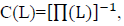
moving average matrix is given by so that the moving average representation (MAR) of Equation 1 is:

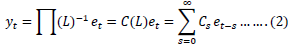
The C_i are determined by the following recurrence relations:

'

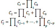Equation 2 is written in terms of the reduced-form shocks. It can be rewritten in terms of the structural shocks as:

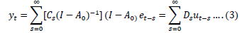
Where For a particular period t + j, Equation 3 may be written as:

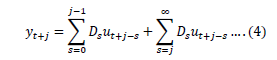
Which represents the historical decomposition . This decomposition has two types of terms. The far right side term represents the expectation of (yt+j) the "base projection" of the vector y, given information available at time t. Because of the structural innovations in the variables after period t, the first term on the right-hand side demonstrates the difference between the actual series and the base projection; that is, it shows that the gap between an actual series and its base projection is the sum of the (weighted) contributions of the structural innovations to the individual series in the analysis. Thus, the actual data at period t + j are the sum of the base projection and the weighted structural innovations to the system variables. As indicated above, these structural innovations are assumed orthogonal to one another.

Data Analysis

A. Unit root test: From the Table 1, We see that all-time series stationary in first order I(1).

Table 1  Unit Roots Test Results, Eviews 10
UNIT ROOT TEST  RESULTS  TABLE (ADF)
Null Hypothesis: the variable has a unit root
	At Level	GAS_PRICE	OIL_EXPORTS__KTOE_	OIL_IMPORTS__KTOE_	OIL_PRICE
With Constant	t-Statistic	-1.9575	2.7284	3.7922	-1.629
	Prob.	0.3037	1.0000	1.0000	0.4588
		n0	n0	n0	n0
With Constant & Trend	t-Statistic	-2.665	-0.6993	-0.2076	-2.4789
	Prob.	0.2557	0.9663	0.9907	0.3363
		n0	n0	n0	n0
Without Constant & Trend	t-Statistic	-0.742	8.6790	9.6853	-0.6667
	Prob.	0.3887	1.0000	1.0000	0.4220
		n0	n0	n0	n0
	At First Difference
		d(GAS_PRICE)	d(OIL_EXPORTS__KTOE_)	d(OIL_IMPORTS__KTOE_)	d(OIL_PRICE)
With Constant	t-Statistic	-8.2271	-5.2925	-5.1225	-6.8224
	Prob.	0.0000	0.0001	0.0001	0.0000
		***	***	***	***
With Constant & Trend	t-Statistic	-8.1215	-5.6027	-6.6045	-6.7411
	Prob.	0.0000	0.0002	0.0000	0.0000
		***	***	***	***
Without Constant & Trend	t-Statistic	-8.2987	-2.6142	-1.2156	-6.908
	Prob.	0.0000	0.0103	0.2015	0.0000
		***	**	n0	***

B. Co-integration: (Table2) shows that the cointegration relationship between variables, because the Trace test indicates 3 cointegrating eqn(s) at the 0.05 level, and Max-eigenvalue test indicates 3 cointegrating eqn(s) at the 0.05 level, denotes rejection of the hypothesis at the 0.05 level.

Table 2  Co-Integration Results, Eviews 10
Date: 06/12/20   Time: 16:51
Sample (adjusted): 1984 2020
Included observations: 37 after adjustments
Trend assumption: Linear deterministic trend
Series: OIL_PRICE OIL_EXPORTS__KTOE_ OIL_IMPORTS__KTOE_ GAS_PRICE D1
Interval with Lags (in first differences): 1 to 3
Unrestricted Rank Test for Cointegration (Trace)
Hypothesized		Trace	0.05
No. of CE(s)	Eigenvalue	Statistic	Critical Value	Prob.**
None *	0.826822	139.6284	69.81889	0.0000
At most 1 *	0.628533	74.75134	47.85613	0.0000
At most 2 *	0.537500	38.11037	29.79707	0.0044
At most 3	0.147309	9.579331	15.49471	0.3145
At most 4	0.094749	3.683077	3.841466	0.0550
Trace test indicates 3 cointegrating eqn(s) at the 0.05 level
denotes refusal of the hypothesis at the level of 0.05
**MacKinnon-Haug-Michelis (1999) p-values
Unrestricted Cointegration Rank Test (Maximum Eigenvalue)
Hypothesized		Max-Eigen	0.05
No. of CE(s)	Eigenvalue	Statistic	Critical Value	Prob.**
None *	0.826822	64.87709	33.87687	0.0000
At most 1 *	0.628533	36.64097	27.58434	0.0026
At most 2 *	0.537500	28.53104	21.13162	0.0038
At most 3	0.147309	5.896254	14.26460	0.6266
At most 4	0.094749	3.683077	3.841466	0.0550
Max-eigenvalue test indicates 3 cointegrating eqn(s) at the 0.05 level
* Denotes dismissal of the hypothesis at the 0.05 level
** P-values MacKinnon-Haug-Michelis (1999)

C. VAR Lag Order Selection Criteria: After Computes various criteria to select the lag order of an unrestricted VAR, We find that the optimal lag (3) in Table 3.

Table 3 Lag Order Selection Criteria Results, Eviews 10
VAR Lag Order Selection Criteria
Endogenous variables: OIL_PRICE OIL_EXPORTS__KTOE_ OIL_IMPORTS__KTOE_ GAS_PRICE D1
Exogenous variables: C
Date: 06/12/20   Time: 15:48
Sample: 1980 2020
Included observations: 38
Lag	LogL	LR	FPE	AIC	SC	HQ
0	-1301.788	NA	5.10e+23	68.77834	68.99381	68.85500
1	-1127.985	292.7209	2.05e+20	60.94660	62.23943*	61.40658
2	-1106.115	31.07827	2.60e+20	61.11134	63.48153	61.95464
3	-1060.548	52.76268*	1.07e+20*	60.02883*	63.47638	61.25544*

D. Test for Autocorrelation: Table 4 shows that p-value equal (0.9150) so We have no Autocorrelation.

Table 4 Breusch-Godfrey Serial Correlation Lm Test Results
Breusch-Godfrey Serial Correlation LM Test:
F-statistic	0.171298	Prob. F(3,33)	0.915
Obs*R-squared	0.628683	Prob. Chi-Square(3)	0.8898

Results

IRF Results Show

1. Positive shocks in the volume of oil exports do not lead to a significant decrease in crude oil prices. During six periods, the Baseline remains inherent to the Baseline + oil export, while the effects of the shock begin slightly in the last four periods (Figure 4-A) This pattern is basically consistent with our model that assumes that the volume of oil exports does not affect much on world oil prices since the oil pricing mechanisms of the exporting countries have changed in favor of other variables (the results of which will be discussed in detail in the coming lines).
2. Positive shocks in the volume of oil imports lead to a decrease in crude oil prices during the first five periods, and the effects of the shock on oil imports remain stable for five other periods and then rise again, during the first five periods the Baseline rises from the (Baseline + oil import) While the effects of the shock begin to settle in the other five periods, the Baseline + oil import curve returns to rise above the Baseline curve until the end of the period (Figure 4-B). This pattern is consistent with our model that assumes that the volume of oil imports affects In oil prices.
3. Positive shocks in natural gas prices This leads to higher demand for crude oil, from the second period, and this is normal due to the slowdown in consumer response, but this response decreases for two subsequent periods, and then rises again clearly, (graph 4 - c) This volatility is due to competition in the global energy markets.
4. The largest response was from the placebo variable (D1), and these responses were elevated in periods of tensions in the oil production areas clearly (Figure 4-D).

Summary and Conclusion

This paper has examined the many variables effects of shocks to oil price within the context of a five-variable vector autoregressive model, in try to know what variable causes the oil price, we examined oil export, oil import, gas price, as substitute good, and dummy variable, as the tension in the oil production regions.

This research has confirmed a long run relationship between the model variable. so We used the functions of Impulse Response to test the response of oil price to oil export, oil import, gas price and dummy variable.

A historical decomposition in Impulse response functions indicate the empirical shocks have effects consistent with those predicted by theory. The IRFs suggest it is important to distinguish between dummy variable shocks and oil import toward oil price.

References

Burbidge, J., & Harrison, A. (1985). An historical decomposition of the great depression to determine the role of money. Journal of Monetary Economics, 16(1), 45-54.

Fackler, J.S., & McMillin, W.D. (1998). Historical decomposition of aggregate demand and supply shocks in a small macro model. Southern Economic Journal, 648-664.

Fan, L., & Li, H. (2015). Volatility analysis and forecasting models of crude oil prices: A review. International Journal of Global Energy Issues, 38(1-3), 5-17.

Jovicic, G., & Kunovac, D. (2017). What is driving inflation and GDP in a small European economy: the case of Croatia (No. 49).

Yan, L. (2012). Analysis of the international oil price fluctuations and its influencing factors.

Yoshino, N., & Alekhina, V. (2019). Empirical analysis of global oil price determinants at the disaggregated level over the last two decades.