Keywords

Economic Scenario Generator (ESG), Vector Autoregressive (VAR), Fundamental Economic Factors, Asset Return.

Introduction

The ability of the pension funds to meet their current or future liabilities depends on the accuracy of estimating the accrued benefits, and thus taking into account all the factors affecting the determination of their future value. Economic factors are considered one of the most important factors affecting the efficiency and effectiveness of the pension funds, and thus affect the ability of those systems to be financially sustainable in the long term.

Projecting the assets and liabilities of the pension funds requires simulation of future economic scenarios. Typically, the economic scenario generator (ESG) produces economic scenarios that manage the economy's evolution, investment returns, inflation rates, and the other factors in a consistent manner. In general, ESG is necessary for producing scenarios, under which changing funding requirements are estimated, especially when there are many factors interacting on both sides of the assets and liabilities (Campbell et al., 2016).

There are a wide range of ESGs that are currently used. Among the few published models for ESG are the Wilkie Models (Wilkie, 1986; Wilkie, 1995; Wilkie, 2011; Mulvey, 1996; Mulvey & Thorlacius, 1998). Under these models, the variables were related to each other in a cascade structure, which means that each subsequent variable in the cascade structure depends only on prior values of the variable and the values of variables that lie above them on the cascade structure.

This paper does not make use of these models. It's needed to reflect the interrelationships between the factors. In this respect, the research has used the vector autoregressive (VAR) model as an alternative approach (it was also recommended in Wilkie & Sahin (2019)). It is one of the stochastic methods that are usually used to predict the interrelated factors and analyze the dynamic mutual influence of these factors. It also avoids the need to develop structural models by treating each of the variables as variables inside the system and dependent on other variables.

This model doesn't have a restrictive cascade structure, allowing each factor to be influenced by any other. It allows the data to recognize a structure between variables, in order to model the economic variables and to fit parameters to the structure (Yakoubov et al., 1999).

ESG for Fundamental Economic Factors

The fundamental factors that are addressed in this paper are the GDP growth rate, short term interest rate, inflation rate, rate of unemployment, growth rate of domestic investment, growth rate of consumption, and salary growth rate. These factors were selected because they can reflect the period-to-period variations in the economy's status and have an indirect impact on the asset returns in a consistent manner. The following table shows the indicator for each factor Table 1.

Table 1 The Indicator For Each Factor
Fundamental Economic Factors	Indicator	Notation
GDP growth rate	quarterly notional GDP growth rate	gdp
Short term interest rate	3-month treasury bill rate	3mtb
Inflation rate	consumer price index	cpi
Unemployment rate		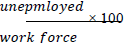unemploy
Domestic investment growth rate	gross domestic investment	dingr
Consumption growth rate	personal consumption expenditures	pconsump
Salary growth rate	rate of salaries increase in Egypt	sgr

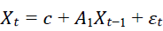
These intertemporal interactions among these factors are modeled using a vector autoregressive (VAR) in which relationships among leading, coincident, and lagging factors can be demonstrated by incorporating lagging variables (For instance, the central bank determines the short-term interest rate after examining the current economic growth, unemployment, and other relevant conditions). Moreover, the VAR(1) model is used to account for the impact of the preceding quarter's values on the evolution of fundamental factors.

Data and Analysis

The generation of scenarios is estimated using quarterly historical dataset of the Egyptian economic factors from 2004/2005Q1 to 2021/2022Q4 (it covers three full economic cycles). This data was collected from the annual reports of the Central Bank of Egypt and the Central Agency for Public Mobilization and Statistics.

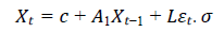
Instead of creating risk-neutral scenarios, the ESG creates real-world scenarios; in order to simulate the future in a realistic manner by generating plausible outcomes based on past observed experience. The status of economic recession or growth is determined by the underlying economic factors jointly. This dependency can be constructed as (Einarsson, 2007):

Where,

X_t⇒acolumn vector with the economic factors during period t
c⇒ a column vector for the intercepts.
A₁⇒ a square matrix of the parameters that describe the linear dependence of economic factors
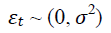
ε_t⇒ a column vector with the terms of error which are assumed to be normally distributed,

Where

The model parameters that were fitted based on historical data are shown in the Table 2 below; along with the standard deviation of the error vector e_t.

Table 2 Paramters Of Var(1) Model
	unemploy	cpi	dingr	gdp	3mtb	pconsump	sgr	c	sigma
unemploy	0.92122	0.021727	0.005181	-0.01809	-0.11439	-0.043058	-0.014645	0.020911	0.006941
cpi	0.076223	0.911031	0.002121	0.093166	-0.16583	-0.019429	-0.072272	0.024668	0.03101
dingr	2.6179	0.4567	0.3313	1.6099	1.0795	1.9134	-0.4653	-0.4359	0.222
gdp	-0.17547	-0.05785	0.03947	0.38022	0.06844	0.03549	0.02987	0.03385	0.01825
3mtb	0.024488	0.128401	-0.00154	0.013741	0.682328	-0.152157	-0.030791	0.02686	0.01033
pconsump	-0.11922	0.05102	-0.01391	0.03798	-0.30219	0.32889	-0.00618	0.06968	0.02079
sgr	-0.27763	0.08202	0.02651	-0.22045	-0.17773	0.08141	0.73697	0.07478	0.03454

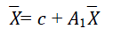
Moreover, the stable values of the economic factors can be derived based on the fitted VAR(1) as follows:

Based on VAR(1), the growth rate of future economic, inflation rate, interest rates, and unemployment rate is expected to be a little bit lower than in the past 17 years. The domestic investment growth rate is expected to be lower in a high percentage than its historical mean Table 3. It is anticipated that consumption will be slightly higher, and the salary growth rate is expected to rise. These implicit expectations serve as useful checkpoints for determining if the model is reasonable in light of the model user's predictions for future economic growth.

Table 3 The Stable Values
Fundamental Factors	Stable value (%)	Historical Data
		Mean (%)	Standard deviation (%)
Real GDP Growth Rate	0.045	0.046	0.024
Consumption Growth Rate	0.050	0.046	0.025
Inflation Rate	0.103	0.110	0.060
Unemployment Rate	0.096	0.104	0.021
Salary Growth Rate	0.138	0.129	0.050
Short Term Interest Rate	0.098	0.103	0.030
Domestic Investment Growth Rate	0.105	0.162	0.249

The error terms of the economic factors which represent the non-systemic component in the model are not independent of each other. Then, it is important to capture the correlation when developing future scenarios Table 4.

Table 4 Var(1) Correlation Matrix Of Error Terms Et
	unemploy	cpi	dingr	gdp	3mtb	pconsump	sgr
unemploy	1	-0.028267	-0.23286	-0.58599	-0.20143	0.04623	0.013439
cpi	-0.02827	1	0.11803	-0.01531	0.15532	-0.2248	-0.003476
dingr	-0.23286	0.118034	1	0.51499	0.0647	-0.27997	-0.059759
gdp	-0.58599	-0.015305	0.51499	1	0.06349	-0.12179	-0.01136
3mtb	-0.20143	0.155325	0.0647	0.06349	1	-0.01785	0.03405
pconsump	0.04623	-0.2248	-0.27997	-0.12179	-0.01785	1	0.01778
sgr	0.01344	-0.003476	-0.05976	-0.01136	0.03405	0.01778	1

In this respect, the economic factors' stochastic scenarios can be determined as (Shang, 2021):

Where,

σ⇒ a column vector of the standard deviation of the error terms
ε_t⇒ a column vector with independent random variables, all of which have a mean of zero.
L ⇒ a lower triangular matrix, allowing the correlation matrix of error term to be decomposed as L×L^T.

Under each scenario, the economic situation is assessed for each quarter to determine whether it's in growth or in recession for accurately analyzing the scenarios, and for generating the returns of assets as well. To predict if the economy is in recession, the following logistic model is used:

Where,

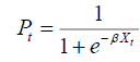
P_t ⇒ the likelihood that the economy will be in recession during period t
β⇒ a row vector providing the model parameters for variables
X_t ⇒ a column vector with the constant term and the economic variables for periods t, and t
-1

ESG for Asset Return

The asset return is a combination of two components: a systemic factor and an idiosyncratic factor. Based on the historical data, the systemic factor is determined by the relationship between asset return and the overall economy, which is driven by key economic factors. As for the idiosyncratic factor, it is determined by each asset class's characteristics (Shang, 2021). The paper has used the assets portfolio of the government social pension fund in Egypt. The fund's historical dataset of asset returns was obtained through the government fund's annual reports, and the fund's cash flows from 1997 to 2021. The amounts of the government pension fund are invested in the National Investment Bank (NIB), treasury bonds (TB), securities & government bonds (Sec & GB), and deposits (Dep). According to Shang & Hossain (2019), Asset return stochastic scenarios can be constructed as:

Where,

y_t ⇒a column vector for all asset classes' returns during period t
a⇒a column vector for the intercepts
Φ⇒a column vector for the parameters to manage the relationship between current return and return for all asset classes during period t
β⇒a matrix that comprises model parameters of all asset classes for the fundamental factors
X_t ⇒a column vector with the economic factors at time t
σε_t ⇒the idiosyncratic part of asset return

Using the above Table 5, we can determine the equations for each asset return; in order to predict the returns for each class accurately.

Table 5 The Relationship Between Asset Returns And The Economic Factors
Lag (Years)	Economic Factors
	1	0	1	0	1	0	1	0	1	0	1	0	1	0
Asset Class	Unemploy		cpi		gdinv		gdp		3mtb		pconsump		sgr
NIB	-0.03	0.01	-0.03	-0.04	-0.01	0	0.04	0.08	-0.04	-0.04	0.15	-0.07	-0.05	-0.04
TB	0.22	-0.14	0.03	0.01	0.04	-0.02	0.08	-0.28	-0.01	0.05	-0.06	-0.32	0.03	-0.04
Sec.&GB	1.17	-0.90	-0.36	-0.49	0.21	0.12	2.30	0.04	-0.28	-0.79	-1.30	0.92	0.34	-0.16
Dep.	1.74	-1.09	0.29	-0.03	-0.12	-0.06	0.04	-0.24	0.10	-0.08	0.55	0.45	-0.15	-0.22

For the NIB investment return

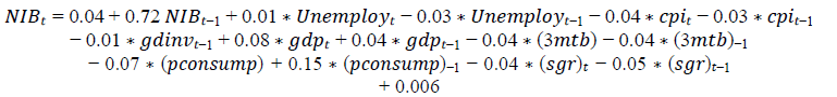
The adjusted R² for this model reached to around 69.2%, which means that the model is able to explain 69% only from the change in the NIB return

For the TB return

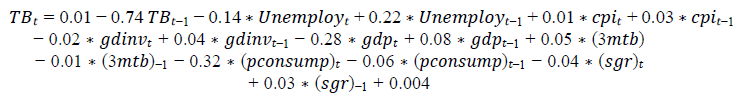
The adjusted R² for this model reached to around 86.8%, which means that the model is strongly able to explain 87% from the change in the TB return

For the Sec.& GB return

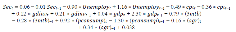
The adjusted R² for this model reached to around 47.4%, which means that the model is able to explain only 47% from the change in the Sec.& GB return

For the Dep. return

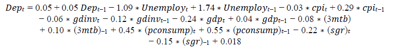
The model have a lowest adjusted R² , where it reached to 23.3%, which means that the model is able to explain 23% only from the change in the Deposits return Figures 1 to 4 show the statistics of 200 generated stochastic scenarios of returns of asset classes, including the expected value, minimum, maximum, and 10^th, 25th, 75^th, and 90^th percentiles.

Conclusions and Recommendations

Asset returns and economic factors don't necessarily correlate linearly. Higher correlation and volatility are frequently observed during economic downturns. Economic asset return scenarios must be further modified to account for the nonlinear relationship. The average growth rate of GDP is 1.5% under the worst scenario and 2.7% under the good scenario. On average, unemployment rates are higher under the bad scenario. Accordingly, interest rates are lower to stimulate the economy.

The yields on treasury bonds, NIB investment, and deposits decrease during economic downturns. Securities & government bonds perform similarly but with varying volatility during recessions. Based on adjusted R² value, the returns of the securities & government bonds and deposit are more influenced by idiosyncratic factors than by economic factor. The bad scenario is not necessarily worse than the good scenario. The main difference between the two scenarios is that under the bad scenario, the economy is moving considerably more slowly than under the good scenario.

Although the factors that are used in this paper are the most common economic factors, other factors can be involved, based on purpose of a model and the features of the economy. It is important to assess each scenario's reasonableness regarding whether basic economic patterns are followed.

References

Campbell, M.P., Christiansen, S., Cox, S.H., Finn, D., Griffin, K., Hooker, N., ... & Pedersen, H. (2016). Economic scenario generators: A practical guide, Society of Actuaries.

Indexed at, Google Scholar, Cross Ref

Einarsson, A. (2007). Stochastic Scenario Generation for the Term Structure of Interest Rates (Doctoral dissertation, Master Thesis, Informatics and Mathematical Modelling, Technical University of Denmark, (DTU).

Indexed at, Google Scholar, Cross Ref

Mulvey, J.M. (1996). Generating scenarios for the Towers Perrin investment system. Interfaces, 26(2), 1-15.

Indexed at, Google Scholar, Cross Ref

Mulvey, J.M., & Thorlacius, A.E. (1998). The Towers Perrin global capital market scenario generation system. Worldwide Asset and Liability Modeling, 10, 286.

Indexed at, Google Scholar

Shang, K., & Hossen, Z. (2019). Liability-driven investment – Benchmark Model, Society of Actuaries.

Shang, K., (2021). Deep Learning for Liability-Driven Investment, Society of Actuaries.

Indexed at, Google Scholar, Cross Ref

Wilkie, A.D. (1984). A stochastic investment model for actuarial use. Transactions of the Faculty of Actuaries, 39, 341-403.

Indexed at, Google Scholar, Cross Ref

Wilkie, A.D. (1995). More on a Stochastic Asset Model for Actuarial Use. British Actuarial Journal, 1(5), 777–964.

Indexed at, Google Scholar, Cross Ref

Wilkie, A.D., & Sahin, S. (2019). Yet more on a stochastic economic model: Part 5: a vector autoregressive (var) model for retail prices and wages. Annals of Actuarial Science, 13(1), 92-108.

Indexed at, Google Scholar, Cross Ref

Yakoubov, Y., Teeger, M., & Duval, D.B. (1999). A stochastic investment model for asset and liability management. In Proceedings of the 9^th International AFIR Colloquium, 237-66.

Indexed at, Google Scholar

Received: 11-Jun-2023 Manuscript No. AAFSJ-23-13686; Editor assigned: 13-Jun-2023, PreQC No. AAFSJ-23-13686(PQ); Reviewed: 27-Jun-2023, QC No. AAFSJ-23-13686; Revised: 14-Jul-2023, Manuscript No. AAFSJ-23-13686(R); Published: 21-Jul-2023