Keywords

Currency Exposure, Wavelet Technique, Food and Beverage Industry

Introduction

Since the abolishment of the Bretton Woods system in 1970s, the issue of exchange rate exposure remains major concern of multinationals and regulators around the globe. Fundamentally, exchange risk becomes one of the important aspects in international asset pricing. The unanticipated change in foreign exchange rate may result in substantial impact to firm’s projected cash flows. Adler & Dumas (1984) defines exchange rate exposure as firm’s sensitivity to any change in foreign currency under a regression framework. A significant number of studies have been conducted to examine exchange rate exposure with large concentration is put under the context of developed economies. However, majority of the studies found minimal level of exposure mainly due to vigorous hedging practices in the region (Abdul Wahab et al., 2017; Suhaimi et al., 2019a). Jorion (1990) reported minimal exposure level with only about 5% of 287 U.S. corporations from 1971 till 1987 were affected by changes in trade weighted index exchange rate. The modest exposure level was due to the widespread hedging activities by the U.S firms.

Under the context of small open economy of Malaysia, firms operating in the country are nonchalantly exposed to exchange risk especially those with substantial foreign sales and imports. The study puts highlight on food and beverage sector, considering that the sector has become one of the major components in Malaysian consumer product industry. Moreover, examining a single sector will provide more meaningful findings as exchange exposure is unique for each industry (Ibrahim, 2008; Abdul Wahab, 2021). Majority of Malaysian firms are net importers of food and beverage goods and services due to the lack of local production, resources and limited alternative energy sources (Abdullah et al., 2018). With this regard, Malaysia imports large amount of raw materials to support its local demands as well as to facilitate its export activities for processed products. Food and beverage corporations were also affected during the Global financial crisis (GFC) 2008 to some extent. We hypothesize that sudden increase and reduction in exchange rate during the GFC has strong influence on the incidence of exposure. The exchange rate exposure tends to be an event specific as a response to the specific financial crisis (Parsley & Popper, 2006; Suhaimi et al., 2019b). Several studies were conducted under the context of Malaysia market. Muller & Verschoor (2007) run large scale study of currency exposure involving 3000 Asian firms including from Malaysia and found that 25% of total firms had significant exposure to the USD with majority of them were highly levered firms. Bartram & Bodnar (2012) examined currency exposure of 4404 non-financial corporations including firms from Malaysia with a duration from July 1994 till December 2006. Interestingly, they found high level of exposure among developing countries and minimal level of exposure among developed countries (US, Canada) due to widespread of hedging use. Specifically, about 15.5% Malaysia firms were significantly exposed to the USD. Abdul Wahab (2017) investigated the impact of Foreign Currency Derivatives (FCD) on the level of exchange risk of 106 non-financial corporations in Malaysia from January 1995 until December 2014. The study reported slightly lower exposure among hedged firms compared to un-hedged firms, signifying the effectiveness of hedging in mitigating exchange risk for short term hedging strategy. Bacha et al., (2013) documented considerably large exposure with about 71% of 158 sample firms had significant exposure to exchange risk. This study argued that the level of economic openness had strong connection with the level of exchange rate exposure. From specification perspective, wavelet analysis in finance is considered relatively new despite of its significant applications in various financial and economic problems such as capital asset pricing model (Masih et al., 2010; Gencay et al., 2005), portfolio allocations (Kim & In, 2010), scaling properties of exchange rate volatility (Gencay et al., 2001) and many more. However, the interest in making importance of wavelet technique in examining the potential time scales exchange rate exposure has not been fully discovered yet. Previous studies only focused on single domain frequency in analyzing exchange rate exposure, ignoring the potential heterogeneity among investors. This is especially true under the imperfect market in which market players demonstrate different expectations and goals in their investment portfolio. Given the heterogeneity in investment interval, wavelet method decomposes return series into different frequencies to further understand the influence of multi-scale investment interval to the level of exposure.

Given all these issues, the first objective of the study is to analyze the multi-scale exchange rate exposure with special emphasis on the food and beverage corporations in Malaysia. The second objective focuses in examining the time varying multi-scale exposure surrounding the Global financial crisis 2008. The organization of the paper is structured as follows; Part 2 explains the data selection and methodology, while section 3 offers discussion on the results. Final part concludes the whole findings and offers direction for future study.

Methodology

Data

For data collection process, the study employs a set of screening criteria. First, the data of firms should span from July 2005 till August 2018. The starting point of data is taken from the date when Malaysia authority decided to de-peg the Malaysian Ringgit from the de facto US dollar peg at MYR 3.80 per USD which took place aftermath the Asian financial crisis 1997. The post de-peg period is opted mainly to avoid multi collinearity problem under the fixed regime. Besides, the effect of exchange rate exposure could be realized better under the floating regime compared to fixed regime. The study uses daily stock returns comprising corporations in Food Producers and Beverage sector as classified by Thompson Reuters Data stream with stringent listing criteria. This enhances the validity of the data extracted for this study. The final sample contains 49 corporations

of food producers and beverage. Daily data of stock returns are extracted to effectively convert our returns series into different classes of frequency. Besides stock returns, the study also collects daily market returns peroxided by FTSE Bursa Malaysia Composite Index as the control market factor. As for exchange rates, four major trading currencies are selected namely the U.S. Dollar (USD), the Great Britain Pound (GBP), the Euro (EUR), and the Japanese Yen (JPY). Direct quotation is used where the value of foreign currency is denominated in term of the Malaysian Ringgit.

Method

In order to ensure the stationary property of each series is taken care of, we transform the original trended series (the stock price (Pt), market index and exchange rates) into stationary series as follows;

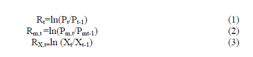
Rt denotes the stock returns, Rm,t represents the market returns while RX,t represents returns for specific bilateral exchange rate i.e., MYR/USD, MYR, EUR, MYR/GBP, MYR/JPY. The next step requires decomposition of each return series into its constituent multi resolution parts through the application of the maximal overlap discrete wavelet transformation (MODWT). MODWT transforms the single frequency domain of stock returns into multi-frequency domains. This provides better understanding on the level of activities occurring during each frequency domain. In this study, a special class of MODWT namely the Daubechies Least Asymmetric wavelet filter of length 8, LA(8) is used to decompose a return series using 5 different scale crystals which are defined as d1 (2-4 days), d2(4-8 days), d3 (8-16 days), d4 (16-32 days) and d5 (32-64 days) (Suhaimi et al., 2019). The decomposed series can be explained as;

j is the number of scale crystals (intervals or frequencies)

k is the number of coefficients in the specified component

?_j,k(t) and ψ_j,k(t) are the father and mother orthogonal wavelet pairs that are given by

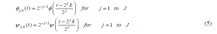
There are several interesting features from this equation. First, the return series is decomposed into the detailed component (mother wavelet) and smooth component (father wavelet). It should be noted that the level of activities occurring within father wavelet should be hypothetically different than that of the detailed part. The coefficients for mother wavelet d_j,k and father wavelet s_j,k are;

s_j,k represents the smooth part of information extracted from return series while the dj,k captures the detailed part within shorter period of time. After extracting the decomposed returns, all the information is combined and regressed under its respective scale. The residual model of Jorion (1990) is employed to effectively capture the level of each scale across different frequency domains. Each model is repeatedly regressed following each scale as follows;

The heart of the study lies on the beta coefficient for each currency (USD, EUR, GBP, JPY). The beta coefficient measures the level of exchange rate exposure and the significance of beta implies the significant impact of exchange rate change on firm value. The positive beta infers better performance during appreciation of foreign currency (favouring exporter) while negative beta implies better performance during depreciation of foreign currency (favouring importer). Under wavelet analysis, identical beta across different time scales signal inexistence of multi-scale nature of currency exposure. On the other hand, different betas across varied scales signify the importance of time scales in exchange risk pricing. For robustness check, the study replicates equation (7) with robust standard error. The study tests the existence of heteroscedasticity problem through a special procedure called Breusch Pagan test for each individual regression. The problem will be handled through Garch(1,1) embedded into the regression model as proposed by Bacha, et al., (2013).

Results and Discussion

Table 1 provides the comprehensive results of the beta coefficients which represent scale-specific exchange risk for all stocks. In ensuring the validity of the results, the analysis is further extended by embedding GARCH (1,1) specification into Jorion (1990) model for firms exhibiting heteroscedasticity problem. Several noteworthy information are shown in Table 1. First, it appears that food and beverage firms show a multi-scale tendency where the extent of beta coefficients for all currencies are changing non-monotonically with the time scale. The magnitudes of positive and negative exposure are increasing from low time scale (high frequency) to high time scale (low frequency).

Table 1 Foreign Exchange Exposure of Food and Beverages firms in Malaysia (OLS with GARCH(1,1)  Specification)
Wavelet Scale	USD				EUR				Global Wald Test
	f	%			f	%			f	%
	{1}	{2}	Mean Beta (Positive)	Mean Beta (Negative)	{3}	{4}	Mean Beta (Positive)	Mean Beta (Negative)	{8}	{9}
D1	9	18.40%	0.1627	-0.1668	7	14%	0.0894	-0.1133	48	98%
D2	8	16.30%	0.099	-0.1255	12	25%	0.0955	-0.0976	48	98%
D3	32	65.30%	0.2519	-0.1333	26	53%	0.1581	-0.1326	49	100%
D4	32	65.30%	0.3433	-0.1339	30	61%	0.1971	-0.191	48	98%
D5	40	81.60%	0.2745	-0.2393	40	81%	0.2954	-0.2288	49	100%
S5	49	100.00%	0.2855	-0.2938	48	98%	0.1815	-0.2942	49	100%
Wavelet Scale	GBP				JPY
	f	%			f	%			R2
	{5}	{6}	Mean Beta (Positive)	Mean Beta (Negative)	{7}	{8}	Mean Beta (Positive)	Mean Beta (Negative)
D1	8	16%	0.0995	-0.0924	12	25%	0.0738	-0.0741	0.0563
D2	11	22%	0.1206	-0.1269	12	25%	0.07	-0.094	0.0704
D3	20	41%	0.1246	-0.1724	22	45%	0.0717	-0.1287	0.1015
D4	32	65%	0.2077	-0.2026	26	53%	0.116	-0.1292	0.1453
D5	40	82%	0.2431	-0.1809	41	84%	0.1821	-0.2044	0.1449
S5	47	96%	0.2906	-0.1735	48	98%	0.1927	-0.1854	0.1705

Table 2 Foreign Exchange Exposure Of Food And Beverages Firms In Malaysia Across The Global Financial Crisis (2008)
Sub-Period GFC	Wavelet Scale	USD					EUR					Wald Test
		f	%			f		%			f		%
		{1}	{2}	Mean Beta (+)	Mean Beta (-)	{3}		{4}	Mean Beta (+)	Mean Beta  (-)	{9}		{10}
Pre-GFC	D1	15	31%	0.7916	-0.712	6		12%	0.2905	-0.3413	46		94%
	D2	13	27%	0.4859	-0.4723	7		14%	0.4172	-0.3435	47		96%
	D3	21	43%	0.9189	-0.4544	20		41%	0.4577	-0.5608	47		96%
	D4	29	59%	0.9553	-0.8716	32		65%	0.4248	-0.7257	48		98%
	D5	44	90%	1.2762	-0.9901	39		80%	1.3528	-0.9078	49		100%
	S5	47	96%	1.7618	-1.9186	48		98%	1.5879	-1.4348	49		100%
Mid-GFC	D1	12	24%	0.5395	-0.5008	6		12%	0.1689	-0.2215	40		82%
	D2	13	27%	0.4502	-0.4791	11		22%	0.2384	-0.2137	44		90%
	D3	17	35%	0.6501	-0.4975	19		39%	0.4055	-0.3337	49		100%
	D4	32	65%	0.8086	-0.6371	28		57%	0.5212	-0.4132	48		98%
	D5	36	73%	0.7783	-0.4581	42		86%	0.7508	-0.3251	49		100%
	S5	47	96%	0.9174	-0.9078	48		98%	0.7732	-0.3302	49		100%
Post-GFC	D1	11	22%	0.1355	-0.1591	10		20%	0.0813	-0.1473	44		90%
	D2	6	12%	0.0953	-0.1678	15		31%	0.1608	-0.1129	46		94%
	D3	22	45%	0.2492	-0.1474	20		41%	0.1654	-0.1473	48		98%
	D4	34	69%	0.3835	-0.099	28		57%	0.1477	-0.2123	48		98%
	D5	36	73%	0.3314	-0.2453	42		86%	0.2025	-0.3078	49		100%
	S5	48	98%	0.3226	-0.4469	48		98%	0.1875	-0.3619	49		100%
Whole Period	D1	9	18%	0.1627	-0.1668	7		14%	0.0894	-0.1133	48		98%
	D2	8	16%	0.099	-0.1255	12		25%	0.0955	-0.0976	48		98%
	D3	32	65%	0.2519	-0.1333	26		53%	0.1581	-0.1326	49		100%
	D4	32	65%	0.3433	-0.1339	30		61%	0.1971	-0.191	48		98%
	D5	40	82%	0.2745	-0.2393	40		82%	0.2954	-0.2288	49		100%
	S5	49	100%	0.2855	-0.2938	48		98%	0.1815	-0.2942	49		100%
Sub-Period GFC	Wavelet Scale	GBP				JPY
		f	%			f		%			R2
		{5}	{6}	Mean Beta (+)	Mean Beta (-)	{7}		{8}	Mean Beta (+)	Mean Beta  (-)
Pre-GFC	D1	8	16%	0.3767	-0.3537	8		16%	0.2491	-0.1792	0.0949
	D2	13	27%	0.3381	-0.3882	12		24%	0.1843	-0.3117	0.1022
	D3	15	31%	0.4079	-0.4073	21		43%	0.3743	-0.2441	0.1737
	D4	20	41%	0.453	-0.3982	28		57%	0.4083	-0.2903	0.2203
	D5	43	88%	0.9931	-0.9588	40		82%	0.7137	-0.4807	0.1832
	S5	47	96%	1.3968	-0.7887	47		96%	0.3905	-0.954	0.173
Mid-GFC	D1	6	12%	0.2364	-0.197	10		20%	0.2031	-0.2	0.1202
	D2	14	29%	0.1871	-0.3606	10		20%	0.2015	-0.2141	0.158
	D3	15	31%	0.1875	-0.3621	24		49%	0.3278	-0.2841	0.2041
	D4	36	73%	0.274	-0.5005	28		57%	0.2936	-0.5475	0.3105
	D5	40	82%	0.4432	-0.3701	39		80%	0.2984	-0.5005	0.3045
	S5	47	96%	0.6149	-0.6577	47		96%	0.3786	-0.5065	0.173
Post-GFC	D1	10	20%	0.1106	-0.132	11		22%	0.0498	-0.0911	0.0337
	D2	8	16%	0.1283	-0.0995	15		31%	0.101	-0.1097	0.0474
	D3	17	35%	0.156	-0.1578	26		53%	0.0458	-0.183	0.0711
	D4	24	49%	0.1697	-0.1808	28		57%	0.1786	-0.1277	0.0847
	D5	40	82%	0.294	-0.2177	39		80%	0.1808	-0.2127	0.3045
	S5	47	96%	0.3096	-0.1386	49		100%	0.2371	-0.2063	0.0929
Whole Period	D1	8	16%	0.0995	-0.0924	12		25%	0.0738	-0.0741	0.0563
	D2	11	22%	0.1206	-0.1269	12		25%	0.07	-0.094	0.0704
	D3	20	41%	0.1246	-0.1724	22		45%	0.0717	-0.1287	0.1015
	D4	32	65%	0.2077	-0.2026	26		53%	0.116	-0.1292	0.1453
	D5	40	82%	0.2431	-0.1809	41		84%	0.1821	-0.2044	0.1449
	S5	47	96%	0.2906	-0.1735	48		98%	0.1927	-0.1854	0.1705

A close visual inspection in Figure 1 and Figure 2 shows that there are upward trends of positive exposure from d1 till d5 and downward trends for negative exposure. The same fashion is also found to the percentage of exposed firms for all currencies. This phenomenon could be explained in the context of the relation between exchange risk and trading holding period. Long term investors face greater amount of risk compared to short term investors. Hence, return for long term investors is expected to be higher to compensate high risk premium. Secondly, there is gradual increase in the value of goodness-of-fit measure (R2), signifying the variability of exchange rates could explain stock returns better at the higher scale component. It seems that explanatory power increases from low scale to higher scale. From here, it could be concluded that the assessment of exchange rate exposure is more relevant at the higher scale, specifically starting from d3 (16-32 days) where percentage of exposed firms reaches above 50%. Third, in term of specific individual currency, it could be clearly seen that USD, EUR, GBP and YEN exhibited higher level of exposure at the high scale and smooth scale (father wavelet). The significant exposure of all stated currencies is no coincidence given by the fact that the four countries are major trading countries with Malaysia.

To specifically conduct the second objective, the study runs sub-period analysis to further understand the behavior of multi-scale exposure surrounding the global financial crisis 2008 (pre, middle and post crisis). Based on Table 2, the identical trend of gradual increase in the level of exposure from low scale to high scale is found across all the sub-periods. Secondly, there is enough evidence that the extent of exposure was peaked during the pre-GFC period followed by the middle of GFC period. The pre-GFC period coincided with de-peg period where the regulator decided to let the de facto peg of the Malaysian Ringgit to the USD to be floated under managed float system. Within this period, Malaysia Ringgit recorded a significant appreciation and causing large fluctuation in exchange returns. The GFC period also recorded high level of exposure, however to a lesser extent than the Asian Financial crisis 1997 as shown by Parsley & Popper (2006); Muller & Verschoor (2007); Bacha, et al., (2013).

Conclusion

The study offers new dimension in investigating the exchange rate exposure of 49 food and beverage corporations in Malaysia through multi-scaling approach. The study applies the Maximal Overlap Discrete Wavelet Transformation (MODWT) technique to effectively decompose all variables into multi-scale orthogonal components. Based on the analysis, there is statistical evidence of multi-scale tendency of exchange rate risk across five levels of scale. The findings are parallel with the existing investment theory which connects the length of investment interval with risk level. It is found that investing in food and beverage stocks within shorter period entails lower level of exchange risk than longer period. Thus, higher risk premium for long term investors should be accompanied with higher returns. From the results, the study suggests that vigorous risk management programs should be focused to manage exchange risk within widened investment horizons. Future research should be concentrated on how hedging practices could affect the level of multi-scale exposure. Further, the analysis could be extended to other industries to get comprehensive overview about the nature of multi-scale exposure of Malaysia corporations.

Acknowledgement

The authors would like to thank the anonymous reviewers of AAFSJ for their useful comments and the financial support granted by Universiti Sains Islam Malaysia under the code: PPPI/FST/0118/051000/16518.

References

1. Abdul, W.H. (2017). Does foreign currency derivative affect the variation of currency exposure: Evidence from Malaysia. Advanced Science Letter, 23(5), 4934-4938.
2. Abdul, W.H., Amir, H.M.A., Mohd, N.N., Yusoff, Y.S & Zainudin, W.N.R.A. (2017). Foreign currency exposure and hedging practices: new evidence from emerging market of ASEAN-4. Advanced Science Letter, 23(5), 4939-4943. Abdul, W.H. (2021). Investigating the influence of shariah compliance on the level of currency exposure across time scales: An application of the wavelet approach. Malaysian Journal of Industrial and Applied Mathematics, 37(1), 1-13.
3. Abdullah, W.M.Z., Zainudin, W.N.R., & Ishak, W.W. (2018). A proposed theoretical model to improve public participation towards renewable energy (RE) development in Malaysia, Advanced Science Letters, 24(11), 8922-8925.
4. Adler, M., & Dumas, B. (1984). Exposure to currency risk: Definition and measurement. Financial Management, 13, 41-50.
5. Bacha, O.I., Mohamad, A., Syed, M.Z.S.R., & Mohd, R.M.E.S. (2013). Foreign exchange exposure and impact of policy switch. The case of Malaysian listed firms. Applied Economics, 45(20), 2974-2984.
6. Bartram, S.M., & Bodnar, G.M. (2012). Crossing the lines: The conditional relation between exchange rate exposure and stock returns in emerging and developed markets. Journal of International Money and Finance, 31, 766–792.
7. Gencay, R., Selcuk, F., & Witcher, B. (2001). Scaling properties of foreign exchange volatility. Physica A., 289, 249-266.
8. Gencay, R., Selcuk, F., & Witcher, B. (2005). Multi scale systematic risk. Journal of International Money and Finance, 24, 55-70.
9. Ibrahim, M.H. (2008). The exchange-rate exposure of sectorial returns: Evidence from Malaysia. International Journal of Economic Perspectives, 2(2), 64-76.
10. Jorion, P. (1990). The exchange rate exposure of US multinationals. Journal of Business, 63, 331-345.
11. Kim, S., & In, F. (2010). Portfolio allocation and the investment horizons: A multi scaling approach. Quantitative Finance, 10, 443-453.
12. Masih, M., Alzahrani, M., & Al-Titi O. (2010). Systematic risk and time scales: New evidence from an application of wavelet approach to the emerging Gulf stock markets, International Review of Financial Analysis, 19, 10-18.
13. Muller, A., & Verschoor, W.F.C. (2007). Asian foreign exchange risk exposure. Journal of Japanese International Economies, 21, 16-37.
14. Parsley, D.C., & Popper, H.A. (2006). Exchange rate pegs and foreign exchange exposure in east and South East Asia. Journal of International Money and Finance, 25, 992-1009.
15. Wan, S.W.N., Abdul, W.H., & Md, R.S. (2019a). Symmetric and asymmetric exchange rate exposure: Evidence from Malaysian non-financial firms. AIP proceedings, 2138, 050028.
16. Wan, S.W. N., Abdul, W.H., & Md, R.S. (2019b). The time-varying exposure of Malaysian non-financial firms using panel and OLS analyses. AIP proceedings, 2138, 050029.
17. Wan, S.W.N., Abdul W.H., & Md, R.S. (2019). Currency exposure and time scales: Application of wavelet method to Malaysian non-financial firms. International Journal of Recent Technology and Engineering, Special Issue 3, 187-192.