Keywords

High-Growth Firms, Gibrat Law, Panel Unit Root Tests, Firm Age, Firm Size.

JEL Classification

L11, C23.

Introduction

Many research papers have highlighted the need to distinguish between the general phenomenon of growth, and the particular ‘high-growth’ (Smallbone et al., 1995; Delmar et al., 2003; Barringer et al., 2005). There is no unique method to measure firm growth throughout a given period (Delmar et al., 2003). There has been an important debate about how to measure firm growth – objective versus subjective approaches; single versus multiple indicators; through sales, assets, employments and so forth (Delmar et al., 2003).

There is no specific method to define Gazelle firm. Birch (e.g. Birch et al., 1995, p. 46) defines High-growth firm (HGF) as “An enterprise establishment which has achieved a minimum of 20% sales growth each year over the interval, starting from a base-year revenue with minimum $100,000.” Hence, the definition of high-growth firm is based on enterprise growing at least at a particular rate (e.g. that firm achieve certain annual growth rate or more for a certain number of years). Another way to define high-growth threshold, Organization for Economic Development (OECD; Ahmad, 2006) proposed defining high-growth firm as enterprises with an average employment growth rate exceeding 20% growth per annum over a 3 year period of time and over 10 or more employees during initial establishment of an enterprise.

ACS, Parsons and Tracy (2008) revisited the concept of gazelle firms for the U.S. Small Business Administration. The result of the study showed that high-growth small and young firms were not the only ones responsible for job creation in the U.S. They concluded that a small number of growing firms with an average age of 25 years were also responsible for a significant amount of job creation and revenue growth in the U.S. They called these type of firms as “high-impact firms” and found that they existed in all industries and almost all regions. They suggested that the policymakers should focus on encouraging these high impact firms rather than trying to increase entrepreneurship, focusing on small and medium scale enterprises or focusing on specific economic sector.

High-growth tends to be associated with a firm’s entrepreneurial behaviour (Stevenson and Jarillo, 1990; Brown et al., 2001) and high-growth firms prioritize growth over profitability. Many attempts have been made to define and identify high-growth firms (HGFs) in the perspective of the advanced economies (Delmar et al., 2003; Eurostat-OECD, 2007; Acs et al., 2008).

Gibrat's Law or the Law of proportionate effect proposed by Gibrat in 1931 states that growth of the firm is independent of its size at a given period of time. Few studies confirm the law and few studies reject the validity of Gibrat's law. Thus, in this study I aim to highlight the significance of testing Gibrat's law in developing countries; it can be noted that most of earlier studies focus on developed markets. Hence in this study, an attempt has been made to validate the Gibrat's Law for emerging markets like India. In the context, this study tries to identify the possibility to accepting or rejecting the validity of Gibrat's law in emerging market.

First, our main objective is to define high-growth firm, there is no specific method to measure firm growth throughout a period of analysis (Delmar et al., 2003). Initially, I create two different group’s namely high-growth and non-high-growth firms, In order to define high-growth firm’s relative sales growth measure is used in the study and the cut-off rate is set at 75%. Specifically, high-growth firms are those firms that have more than 75% sales growth from 2010 to 2014. Secondly testing of Gibrat law based on the age of the firm for which five different groups have been created based on the age of the firms and two set of groups they are high-growth and non-high-growth firms. Finally, I use quantile regression, which provides a complete estimation of the growth distribution of high-growth and non-high-growth firms.

Empirical regression model has been able to explain how the growth of the firm is influenced by firm’s age, liquidity ratio and net working capital. In the analysis reported here, I make less restrictive assumptions in analysing the complete conditional distribution of firm growth rates. Using quantile regressions, I examine to what extent selected co-variants may affect the conditional distribution of growth rates. In sum the main contribution of this paper are the following: (1) Sales (firm size) is considered as the measure to define high-growth firm (2) as far as testing Gibrat law is concerned this is the first attempt to validate the law in Indian market (3) the present research validates the Gibrat law by considering age of the firms and also using quantile regression an attempt has been made to understand how firm’s age, liquidity ratio and net working capital affect the firm growth for high-growth and non-high-growth firms.

Theoretical Development

As per Mansfield (1962) Gibrat’s law can be tested in following three ways: (1) for all companies within a given market in the considered time interval including also the companies which do not survive (2) only for surviving companies in the regarded period; (3) only for firms large enough to reach the minimum efficient scale (MES). When differentiating firms by size, one can observe that deviations from the law become less with growing firm size (Evans, 1987; Hall, 1987). Analysing large firms, some studies cannot reject the law (Hall, 1987). The majority of analysis was carried out with data from the manufacturing sector. Audretsch et al. (2004) analysed “Gibrat law” for the Dutch hospitality industry with the similar approaches applied in this study and the result of the study showed that Gibrat law is accepted in 4 out of 15 cases for five different branches.

The majority of the studies reject the validity of the law (e.g. Wagner, 1992; Reid, 1995; Weiss, 1998; Audretsch et al., 1999). Wagner (1992) tests the law for manufacturing companies in lower Saxony with the time period of 1978 to 1989. The outcome reveals that “Gibrat’s law” holds for all the companies included in the study due to the point that the interference phase in the development equation employs a first-order autoregressive process.

This reflects that the growth process of the company will take a certain probabilistic approach, i.e., it is possible that company is noticing above average growth in one period will grow considerably in the following period.

Moreno and Casillas (2000) point out that high-growth firms exhibit two main characteristics: (1) they experience a powerful growth in size, which in majority of the cases leads them to maximize as much as double their initial size; and (2) this fast growth takes place in a very short span of period, which ranges between four to five years (regardless of what measures have been used to determine firm growth rate, i.e. growth in sales, employee headcount and so on). Mason and Brown (2013) suggest that regulators and policy makers should be focused towards promoting high-growth and start-up firms. Based on the empirical study, HGF can be of any size.

Whereas small companies are overrepresented in the population of HGFs, large companies can also play an important role in creating the jobs (Coad et al., 2012). Coad and H¨olzl (2009) do observe some persistence in the top tail of the growth distribution with small high-growth firms displaying negative autocorrelation, whereas large and established companies achieving smoother dynamics. Conversely, Capasso et al. (2013) Conclude that consistent outperformers are more often present among micro firms. Several theories have tried to determine the main elements underlying firm growth. They can be divided into two main aspects: the first deals with the impact of firm size and age on growth, while the second aspect deals with the impact of variables like strategy, entrepreneurial and firm’s manager’s characteristics.

Firm performance Gibrat law has an extensive background in economics (Gibrat, 1931; Ijiri and Simon, 1964; Levinthal, 1991). The result of numerous empirical studies in that firm growth decreases with size (Geroski, 1995; Caves, 1998). This represents a "stylized fact" in the view of few authors (Acs and Audretsch, 1990). The negative correlation between growth and size, one the other hand, contradicts "Gibrat's law", according to which growth follows a random walk approach and is not correlated with the firm size.

Since the early sixties, numerous empirical studies have been conducted to analyse the applicability of "Gibrat's law" (for extensive surveys: Wagner, 1994; Geroski, 1995; Carre, 1996; Sutton, 1997; Caves, 1998).

The Law and Its Empirical Evidence

The majority of the studies focus on testing the law and its proportionate effects which are also known as Gibrat's Law (Gibrat, 1931).One significant study into the determinants of high-growth companies compared to marginal survival (Cooper et al., 1994) showed that chances of survival and high-growth were positively associated with having an advanced stage of education, greater industry-specific know-how, and greater preliminary economic resources.

The result of numerous empirical studies is that firm growth decreases with size (Geroski, 1995; Caves, 1998). This represents a “stylized fact” in the opinion of some authors (Acs and Audretsch, 1990). The negative correlation between growth and size, however, contradicts “Gibrat’s law”, according to which growth follows a random walk independently of firm size. Since the early sixties, numerous empirical studies have been conducted to examine the validity of “Gibrat’s law” (for comprehensive surveys see Wagner, 1992; Geroski, 1995; Schmidt, 1995; Klomp, 1996; Sutton, 1997; Caves, 1998).

Storey (1994) provides an outline of the many aspects considered by researchers prior to 1994 and indicates that among small companies, there are six aspects of significance: company age, dimension, market, sector/market places, legal form, location and possession. Storey notices that previous researchers have revealed that age is inversely related to growth that is older companies develop more gradually than young companies. As already noted, empirical research has demonstrated that smaller firms grow at greater rather than larger firms. However, Storey notices that Evans (1987) and Hall (1986) were the first to show that Gibrat's law did not hold for U.S. firm. Many studies which have exclusively focused on investigating the growth of firms in the Indian context (Das, 1995; Shanmugam and Bhaduri, 2002).

Only a few studies that had analysed the growth pattern of firms in developing countries. For example, Oliveira and Fortunato (2006) have examined the growth pattern of Portuguese manufacturing firms. Kumar (1982), Kaur (1997), Shanmugam and Bhaduri (2002) had investigated the dynamics of firm size distributions of Indian manufacturing firms either in the pre or initial years of liberalization. Further, review shows that no comprehensive study was found in India, which essentially covers the post-liberalization period of 15 years, i.e., from 1991-1992 to 2005-2006, analysing the pattern of corporate growth both firm wise and industry wise. Finally the vastly changing institutional and operating environment of developing countries (Das, 1995); widened and deepened financial markets including the capital market (Kakani et al., 2001 and Shanmugam and Bhaduri, 2002), more flexibility to corporate managers in choosing their expansion path, etc., are a few emerging elements that have provoked the need to carry out this study. Thus, keeping into consideration all these facts, this study was carried out. The objective of this study is to examine the pattern of corporate growth in India during the period 2010 to 2014.

Deriving Hypothesis and Methodology

Firm size and age have been viewed as the determinants of firm growth. The Theory of Learning (Jovanovic, 1982) emphasizes the role played by organizational learning, through the firm’s managers, in the creating a perception and expectations pertaining to the performance of the firm. Jovanovic’s (1982) model suggests that younger firms will have higher growth rates and also the model suggest that the growth of the firm decreases with firm age (Evans, 1987). As per theory of learning younger firms will have higher growth rates when compared to older or established firms, as older firms try to optimize their size in order to increase the efficiency which will show fewer changes in the size of the older firms (Fariñas and Moreno, 1997). Yet, another study of Yasuda (2005) showed a negative effect on firm size and growth. The above explained instances will raise the question does Gibrat law hold good When it is validated separately based on the age of the firms?

In order to address this issue, five different groups have been created separately based on the age of the firm and in the present study, the Gibrat law is tested only for high-growth firms. Levinthal (1991) has made a key assumption in which he mentioned that the firm growth is a random walk. The law of proportionate effect, which views whether the firm growth is independent of its size, has obtained a considerable interest in the literature.

Testing of this law amounts to a consideration of whether firms converge in the direction of a geometric mean size over time, more formally growth can occur through the random walk process:

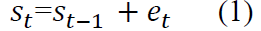
Where S_t is the logarithm of a firm size which is measured in terms of revenue from sales and services (Sales) at time t and e_t is a random shock (additive in logs) with mean u and variance as σ². To test the whether the growth is random walk; unit root test is applied in the study.

Methodology

The main objective of the paper is to arrive at high-growth firms and test the validity of Gibrat’s Law for Indian manufacturing Industry. Various econometric methods have been applied to test for the Law of Proportionate Effects validity. In this sense, it has been argued that the univariable unit root tests possess low power against panel unit root tests alternatives (Aslan, 2008; Diebold and Nerlove, 1990). In this sense, many panel unit root tests have been developed with an emphasis on the attempt to combine information from the time series dimension with information obtained from the cross-sectional dimension (Asteriou and Hall, 2007). Given the nature of the objective, Unit root I’m Pesaran-Shin (1995) (Further it will be referred as IPS) and Levin and Lin (1993) (Further it will be referred as LLC) is one of the better statistical instrument as suggested by Pedroni (1999) when using time series unbalanced data. The basic panel data model with a first-order autoregressive element is considered in the study which is expressed as follows:

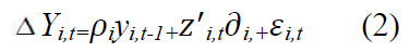
Where I=1…, N panel indexes; t=1 (time)…... T_i; Y_i,t is the variable being tested; and ε_i,t is a stationary error term. The T_i;represents panel specific means and time trend (fixed effects). – Pesaran Shin unit root test is primarily used to test the random the law, as per the test null hypothesis (H0) are panels contain unit root test where alternative hypothesis (Ha) panels are stationary or do not contain a unit root. Considering the above explanation, following model can be derived:

Where Y is a measure of the size (sales) of the firm I=1 (time), N and t=1..., T and e_i,t is the random shock which is all unanticipated shocks which determine the growth of the firm. Primarily, the null hypothesis that Y_i,t contains a unit root (and therefore a stochastic trend) comprises testing p=0 against the alternative hypothesis which rejects the Gibrat law.
In, Levin-Lin-Chu (LLC) all panels considers autoregressive parameters, LLC test is used based on the following model:

Under the null hypothesis of a unit root test, y_i,t is non-stationary, will have a non-standard distribution that depends on the part of term.

Data Description and Measurement Of Firm Age

The data used in this study came from the ProwessIQ released by Centre for monitoring Indian Economy Pvt Ltd, a well-known and widely used commercial database which provides the information on the financial performance of Indian companies. ProwessIQ contains a detailed balance sheet and income statement information of firms in India of all sector of activity. The period of time covered in the study is from 2010 to 2014: this period is used to determine the high-growth firms. In order to determine high-growth firm compound annual growth rate is determined to identify two sets of groups namely: (a) High-growth firm

(b) Non-high-growth firm. The primary objective is to identify two categories of manufacturing firms they are: HGF and NHGF. There is no specific method to measure firm growth throughout a period of analysis (Delmar et al., 2003). Since the source of data was based on the financial reports, I have employed sales growth, similar to the earlier study (Megaravalli, 2017; Baum et al., 2001; Lumpkin and Dess, 2001).

Sales growth by taking relative growth measure and compound annual growth rate of the firms throughout the period 2010-2014. Specifically, I began the analysis by setting following criteria’s:

1. HGFs are those firms that have more than 75% sales growth from 2010 to 2014.

2. NGFs are those firms which do not have the minimum growth rate of 75% in the selected period.

3. They are not distressed at the time of the survey.

According to the above criteria, 102 firms are identified as high-growth firms, which is 5.31% of the total sample size of 1908 firms. Table 1 shows the overview of the total sample of the firms and also shows the industry wise distribution of high-growth firms. Present empirical research is based on a sample of 1.908 firms of Indian manufacturing industry, for the purpose of the following segments were picked randomly, those firms are:

Table 1: Industry Distribution Of High-Growth Firms
S. No.	Industry Description	Number of Firms	Number of HGFs	% of HGFs
1	Agriculture machinery, aluminium, air conditioners & refrigerators, bakery, boilers & turbines, beer & alcohol, books & cards	81	7	8.64
2	Castings & forgings, cloth, commercial vehicle, coffee, ceramic, Cement, cocoa & confectionery, caustic soda	122	10	8.20
3	Cotton & blended yarn, cosmetics & toiletries, computers & Peripherals, communication equipment, consumer electronics, copper	116	10	8.62
4	Diversified, drugs & pharmaceuticals, dyes & pigments, diversified machinery, dairy products, diversified cotton Textiles	219	5	2.28
5	Fertilisers, ferro-alloys, footwear, floriculture, engines	40	1	2.50
6	Gems & jewellery, general purpose machinery, generators, transformers & switchgears	96	3	3.13
7	Glass & glassware, inorganic chemicals, granite, industrial machinery	50	2	4.00
8	Machine tools, media print, lubricants, metal, man-made filaments & fibres, marine foods	113	3	2.65
9	Mining & construction, milling products, organic chemicals, manufactured articles, electrical machinery	75	3	4.00
10	Other: electronics, automobile ancillary, agriculture products, textiles, chemicals, non-ferrous metals, domestic appliance, industrial machinery, leather, transport	381	20	5.25
11	Polymers, plastic, polymers, processed food, poultry, paper & news print, pig iron, pesticides, paints & varnishes, passenger vehicle	219	12	5.48
12	Sponge iron, steel, steel pipes & tubes, readymade garments, sugar, rubber, starches, batteries, refinery	261	20	7.66
13	Wood, tyres & tubes, vegetable oils, tea, trading, wires & cables, textile, two & three wheelers, tobacco	135	6	4.44
	Total	1908	102	5.35

The distribution of high-growth firm is different among the industries the main reason could be because of differences in the life cycle of the firms, intensity of technology and other micro and macroeconomic factors.

Measurement Of Firm Age

Firm age was determined by the difference between firms year of incorporation and initial period considered in the study which is 2010. Thus, the variable representing firm age is as follows:

Firm age=(Initial period considered in the study) 2010 - Year of Incorporation

The below table shows the composition of high-growth and non-high-growth firms based on the age of the firm. Table 2 gives the overview of the distribution of growth rate and summary of age wise growth rate.

Table 2: Composition Of High-Growth Firms By Age Of The Firms
	Age of Firm	Number of irms	Number of HGFs	% of HGFs
Group 1	0-4	277	42	15.16
Group 2	5-8	288	15	5.21
Group 3	9-12	269	16	5.95
Group 4	13-16	542	14	2.58
Group 5	17-19	532	15	2.82
	Total	1908	102	5.35

After distinguishing five different groups based on the age of the firm, the same composition is used to test the Gibrat law. The composition structure shows that younger and start-up firms (0-4) have a higher number of high-growth firms.

IQAfter distinguishing five different groups based on the age of the firm, the same composition is used to test the Gibrat law. The composition structure shows that younger and start-up firms (0-4) have a higher number of high-growth firms.

Results

Table 3: Summary Statistics Of Sales (Each Year) And Growth Rates
Sales	Mean	S.D	10%	25%	75%	90%	Obs
2010	3362.76	12878.05	46.40	225.60	2359	6322.20	1908
2011	4153.67	16436.57	59.10	269.50	2807.10	7285.40	1908
2012	4645.26	18528.90	72.30	274.05	3136.50	8576.90	1908
2013	5140.76	22168.75	61.40	282.65	3343.70	9283.10	1908
2014	5330.29	22625.80	61.50	286.75	3409.45	9553.70	1908
Sales Growth
2010-2011	873.68	504.51	187	435	1306.5	1584	1908
2011-2012	865.72	495.67	181	463.5	1293.5	1564	1908
2012-2013	888.04	506.45	183	464.5	1324.5	1591	1908
2013-2014	482.55	251.62	184	393	631.5	902	1908

Note: Table 4 shows the summary statistics of firm size and growth rates

Table 3 shows an overview of sales trend from 2010 to 2014 and sales growth for the respective years. The highest mean value of sales is 5330.29 in 2014. This shows that the growth has been slightly increasing from 2010, which shows a positive bullish trend of the firms. Further, sales growth is calculated based on compound annual growth rate of the firm. The results of sales growth show that the mean of the sales growth rate has shown a downward trend for the first two years and again shown an upward trend and again downward trend, which shows that the growth rate of the firm is slightly volatile.

Firm Size Distribution

Kernel density function is distributed symmetrically around 0 and 1 over the defined range and reflects as kernel density function (Silverman, 1986). Figure 1 contains the graphical representation of sales expressed in terms of compound annual growth rate from the period 2010 to 2014. A right skew curve which is also found in the work of (Almus, 2000). The extreme left side curve also indicates that the variance of the firm size increases over time. In the view of this result, now it is possible to test the Gibrat law which argues that firm size is only determined by random walk and every firm have the similar growth.

From the Figure 1 emphasizes the fact that the term firm growth (sales growth) does not imply that all high-growth firm have positive growth, but there are also many firms which experience negative growth rates. Age wise analysis of growth.

The age of the firm also plays a vital role in the corporate growth. Thus an attempt is made in the present study to examine the growth pattern of selected firm’s and there are wise distributions of growth. Table 3 shows the distribution of firms under age groups on the basis of compounded growth rate of net sales from the year 2010 to 2014. Table 4 shows that a maximum number of firms (943) which is constituting 70% of total firms were having the growth rate between 0 to 30% and 210 firms which are 15% of the total firms have the growth rate of 30 to 50 %.

Only small number of firms have the growth rate of more than 280% in that younger or start-up firm (0 to 4 years) have high-growth rates, which also support the previous work, Younger firms are found to grow faster than older (Glancey, 1998).

Unit Root Test Results

Table 4:  Compounded Growth Rate In Net Sales By Firm’s Age
Growth rate (%)	0 to 4	5 to 8	9 to 12	13 to 16	17 to 19	Total
0-30	13	148	153	311	318	943
30-50	38	31	24	66	51	210
50-80	28	16	11	16	18	89
80-120	14	7	8	6	8	43
120-160	7	1	1	4	1	14
160-200	3	1	1		2	7
200-240	2	2		2		6
240-280		1	1			2
>280	12	1	3	2	3	21
Total	117	208	202	407	401	1335
Mean	14.625	23.11111	25.25	58.14286	57.28571
SD	12.46638	47.92036	52.21043	113.8192	116.3009

Table 5: Panel Unit Root Test (Ips Test)
	Groups (Age)	No of Firms	IPS Test Without time trend	IPS Test With time trend
1	0-4
	HGF	42	-3.1878***	-13.8823***
	NHGF	235	-7.4821***	-5.7348***
2	5-8
	HGF	15	4.4237	2.2382
	NHGF	273	-10.2358***	-7.2085***
3	9-12
	HGF	16	-0.9202	-1.0375
	NHGF	253	-7.9209***	-6.2374***
4	13-16
	HGF	14	-9.1508***	-7.2602***
	NHGF	528	-21.6402***	-21.9329***
5	17-19
	HGF	15	-2.0451**	-1.7076**
	NHGF	517	-17.7678***	-16.7218***

Table 6: Panel Unit Root Test (Levin And Lin Test)
	Groups (Age)	No of Firms	Adjusted Statistic Without time trend	Adjusted Statistic With time trend
1	0-4
	HGF	42	-6.6410***	6.6825***
	NHGF	235	-20.6943***	-42.3588***
2	5-8
	HGF	15	-6.4357***	-9.7391***
	NHGF	273	-14.9227***	-13.8165***
3	9-12
	HGF	16	-3.5120 ***	-3.8254***
	NHGF	253	-13.9981***	-12.0465***
4	13-16
	HGF	14	-1.0215	-4.6968***
	NHGF	528	-21.1386***	-21.8985***
5	17-19
	HGF	15	-2.4741***	-7.9006***
	NHGF	517	-19.0697***	-18.6135***

Tables 5 and 6 shows the results of applying the panel unit root test to firm’s age level and as per high-growth and non-high growth firm’s (subgroup level) where I applied Im – Pesaran – Shin and Levin and Lin. In almost every instance the null hypothesis supporting Gibrat law is rejected. Table 4 provides the test statistics based on all firm’s age and growth classification (high-growth and non-high-growth firms) during the year 2010 to 2014 period, and the unit root hypothesis is not rejected in only four out of 10 groups (five groups based on age group and two sub groups based on growth), For the age group 5 to 8 and 9 to 12 and these were high-growth firms, which shows that Gibrat law is accepted which means the growth for these firms follows a random walk approach.

In Table 6, the Gibrat law was tested using LLC test and again in most of the cases, the null hypothesis was rejected in all the groups except one. For the age group 13 to 16 where null hypothesis supporting Gibrat law failed to reject.

Quantile Regression

Table 7: Results Of The Quantile Regression, With Industry Dummy
	Variables	q.10	q.25	q.50	q.75	q.90
High-growth firms	Firm Age	0.0319***	0.0203	0.0328	0.0311	0.2***
		(0.00)	(0.26)	(0.48)	(0.43)	(0.00)
	Liquidity ratio	0.0038***	0.0043***	0.0056***	0.0061***	0.0061***
		(0.00)	(0.00)	(0.00)	(0.00)	(0.00)
	Net working capital	-0.0008***	-0.0007***	-0.0006**	-0.0006***	-0.0005***
		(0.00)	(0.00***)	(0.03)	(0.01)	(0.00)
No of Obs: 102	Pseudo R2	0.5055	0.5132	0.5983	0.7648	0.8925
Non-high-growth firms	Firm Age	-0.0039	-0.0012	-0.0022	-0.0045***	-0.0082***
		(0.129)	(0.439)	(0.098)	(0.00)	(0.00)
	Liquidity ratio	-0.0002*	-0.0002***	-0.00002	0.000014	0.00016
		(0.084)	(0.00)	(0.767)	(0.824)	(0.116)
	Net working capital	5.49	-4.09	-3.02	-2.54	-6.82
		(0.469)	(0.395)	(0.447)	(0.518)	(0.991)
No of Obs: 1806	Pseudo R2	0.175	0.1014	0.0618	0.079	0.1376

The results of the first basic quantile regression are shown in Table 7. The estimated quantiles are respectively the 10^th, 25^th, 50^th (or median), 75^th and 90^th quantile.In line with earlier results, the negative effect of age for non-high-growth firm, indicating that learning effects seem to be at work for young firms, as suggested by Jovanovic’s learning models and the results can be also found in previous works (Mazzucato and Parris, 2014; Amato & Burson, 2007). For high-growth firms, there is a positive effect in lower quantile which is also found in earlier work (Papadogans, 2007).The liquidity ratio for high-growth firms is positive shows that as firms liquidity position increases the percentage of growth also increases. Cash at bank etc. This means that growth of the company is positively related to firm growth. Good liquidity position also shows the efficiency of the firms in managing its working capital management. The increase in liquidity ratio reveals the capability of the company to pay off its short-term requirement. On the other side, for non-high growth firms, lower quantile showed a negative effect.

For high-growth firms negative net working capital shows the negative effect which is also found in previous studies (Mohamad and Saad, 2010; Afza and Nazir, 2007).

Conclusion

This study has tested the Gibrat’s law for five different groups which were identified as per the age of the firms, additionally in this paper an attempt has been made to also test the Gibrat’s law for high-growth and non-high-growth firms for manufacturing firms in India covering the 2010-2014 period, and finds strong evidence that Gibrat’s law can be conclusively rejected, This result is also found in the work of (Boutabba & Lardic, 2017) where Gibrat law is rejected for selected manufacturing industry. Various analysis using different groups and growth classification, and two different panel unit root tests reached a fairly unanimous conclusion that Gibrat law is not valid for Indian manufacturing industry. Finally, I applied quantile regression to understand how firm age, liquidity ratio and working capital effect these two group of firms (high-growth and non-high-growth), the results of the study suggest that firm age positively affect the growth of the firm for high-growth firms and negatively affect for non-high-growth is also supported in the previous studies (Yasuda and Takehiko, 2005) and liquidity ratio and working capital is positively affected for high-growth firms. In contrast Audretsch et al. (2004) analysed “Gibrat law” for the Dutch hospitality industry with the similar approaches applied in this study. The Gibrat law is accepted in 4 out of 15 cases for five different branches. The majority of the studies reject the validity of the law (e.g. Wagner, 1992; Reid, 1995; Weiss, 1998; Audretsch et al., 1999).

References

1. Acs, Z.J. & Audretsch, D.B. (1990). The determinants of small-firm growth in US manufacturing. Applied Economics, 22(2), 143-153.
2. ACS, Z.J., Parsons, W. & Tracy, S. (2008). High-impact firms: Gazelles revisited. Washington, DC.
3. Afza, T. & Nazir, M.S. (2007). Is it better to be aggressive or conservative in managing working capital? Journal of Quality and Technology Management, 3(2), 11-21.
4. Ahmad, N. (2006). A proposed framework for business demography indicators.
5. Acs, Z.J. & Audretsch, D.B. (1990). The determinants of small-firm growth in US manufacturing. Applied Economics, 22(2), 143-153.
6. Almus, M. (2000). Testing" Gibrat's Law" for young firms – Empirical results for west Germany. Small Business Economics, 15(1), 1-12.
7. Amato, L.H. & Burson, T.E. (2007). The effects of firm size on profit rates in the financial services. Journal of Economics and Economic Education Research, 8(1), 67.
8. Aslan, A. (2008). Testing Gibrat’s law: Empirical evidence from panel unit root tests of Turkish firms.
9. Asteriou, D. & Hall, S.G. (2007). Applied econometrics: A modern approach, revised edition. Hampshire: Palgrave Macmillan.
10. Audretsch, D.B., Santarelli, E. & Vivarelli, M. (1999). Start-up size and industrial dynamics: Some evidence from Italian manufacturing. International Journal of Industrial Organization, 17(7), 965-983.
11. Audretsch, D.B., Klomp, L., Santarelli, E. & Thurik, A.R. (2004). Gibrat's law: Are the services different? Review of Industrial Organization, 24(3), 301-324.
12. Barringer, B.R., Jones, F.F. & Neubaum, D.O. (2005). A quantitative content analysis of the characteristics of rapid-growth firms and their founders. Journal of Business Venturing, 20(5), 663-687.
13. Baum, J.R., Locke, E.A. & Smith, K.G. (2001). A multidimensional model of venture growth. Academy of Management Journal, 44(2), 292-303.
14. Boutabba, M.A. & Lardic, S. (2017). Does European primary aluminum sector is exposed to carbon leakage? New insights from rolling analysis. Economics Bulletin, 37(1), 614-618.
15. Birch, D.L., Haggerty, A. & Parsons, W. (1995). Who’s creating jobs? Boston, MA: Cognetics Inc.
16. Brown, G.D. & Gordon, S. (2003). Fungal β-glucans and mammalian immunity. Immunity, 19(3), 311-315.
17. Caves, R.E. (1998). Industrial organization and new findings on the turnover and mobility of firms. Journal of Economic Literature, 36(4), 1947-1982.
18. Capasso, M., Cefis, E. & Frenken, K.(2013). On the existence of persistently outperforming firms. Industrial and Corporate Change, 23(4), 997-1036.
19. Coad, A. & Hölzl, W. (2009). On the autocorrelation of growth rates. Journal of Industry, Competition and Trade, 9(2), 139-166.
20. Coad, A. & Broekel, T. (2012). Firm growth and productivity growth: Evidence from a panel VAR. Applied Economics, 44(10), 1251-1269.
21. Cooper, A.C., Gimeno-Gascon, F.J. & Woo, C.Y. (1994). Initial human and financial capital as predictors of new venture performance. Journal of Business Venturing, 9(5), 371-395.
22. Das, S. (1995). Size, age and firm growth in an infant industry: The computer hardware industry in India. International Journal of Industrial Organization, 13(1), 111-126.
23. Delmar, F., Davidsson, P. & Gartner, W.B. (2003). Arriving at the high-growth firm. Journal of Business Venturing, 18(2), 189-216.
24. Diebold, F.X. & Nerlove, M.(1988). Unit roots in economic time series: A selective survey (No. 49). Board of Governors of the Federal Reserve System (US).
25. Eurostat, O.E.C.D. (2007). Eurostat-OECD manual on business demography statistics.
26. Evans, D.S. (1987). Tests of alternative theories of firm growth. Journal of Political Economy, 95(4), 657-674.
27. Fariñas, J.C. & Moreno, L. (1997). Size, age and growth: An application. Fundación Empresa Pública.
28. Geroski, P.A. & Geroski, P.A. (1995). Innovation and competitive advantage (No. 159). Gerosky: Organisation for Economic Co-operation and Development.
29. Geroski, P.A. (2002). The growth of firms in theory and in practice. Competence, Governance and Entrepreneurship-Advances in Economic Strategy Research.
30. Gibrat, R. (1931). Les inégalités économiques: applications: aux inégalitês des richesses, à la concentration des entreprises, aux population’s des villes, aux statistiques des familles, etc: d'une loi nouvelle: la loi de l'effet proportionnel. Librairie du Recueil Sirey.
31. Glancey, K. (1998). Determinants of growth and profitability in small entrepreneurial firms. International Journal of Entrepreneurial Behavior & Research, 4(1), 18-27.
32. Hall, B.H. (1986). The relationship between firm size and firm growth in the US manufacturing sector.
33. Ijiri, Y. & Simon, H.A. (1964). Business firm growth and size. The American Economic Review, 77-89.
34. Jovanovic, B. (1982). Selection and the evolution of industry. Econometrica: Journal of the Econometric Society, 649-670.
35. Littunen, H. & Tohmo, T. (2003). The high-growth in new metal-based manufacturing and business service firms in Finland. Small Business Economics, 21(2), 187-200.
36. Mansfield, E. (1962). Entry, Gibrat's law, innovation and the growth of firms. The American Economic Review, 52(5), 1023-1051.
37. Kakani, R.K., Saha, B. & Reddy, V.N. (2001). Determinants of financial performance of Indian corporate sector in the post-liberalization era: An exploratory study.
38. Kaur, K. (1997). Growth and firm size-evidence from the Indian firms. Indian Economic Journal, 45(2), 121.
39. Klomp, L.(1996). Empirical studies in the hospitality sector: Empirische studies over de Horeca. Offsetdrukkerij Ridderprint.
40. Kumar, M.S. (1985). Growth, acquisition activity and firm size: Evidence from the United Kingdom. The Journal of Industrial Economics, 327-338.
41. Levinthal, D.A. (1991). Random walks and organizational mortality. Administrative Science Quarterly, 397-420.
42. Levin, A., Lin, C.F. & Chu, C.S.J. (2002). Unit root tests in panel data: asymptotic and finite-sample properties. Journal of Econometrics, 108(1), 1-24.
43. Lumpkin, G.T. & Dess, G.G. (2001). Linking two dimensions of entrepreneurial orientation to firm performance: The moderating role of environment and industry life cycle. Journal of Business Venturing, 16(5), 429-451.
44. Mansfield, E. (1962). Entry, Gibrat's law, innovation and the growth of firms. The American Economic Review, 52(5), 1023-1051.
45. Mason, C. & Brown, R. (2013). Creating good public policy to support high-growth firms. Small Business Economics, 40(2), 211-225.
46. Mazzucato, M. & Parris, S. (2014). Heterogeneity, R&D and growth: A quantile regression approach. Small Business Economics, 43(1).
47. Megarvalli, A. (2017). Estimating growth of SMES using a logit model: Evidence from manufacturing companies in Italy. Management Science Letters, 7(3), 125-134.
48. Mohamad, N.E.A.B. & Saad, N.B.M. (2010). Working capital management: The effect of market valuation and profitability in Malaysia. International Journal of Business and Management, 5(11), 140.
49. Moreno, A.M. & Casillas, J.C. (2000). High-growth enterprises (Gazelles): An conceptual framework. Departamento de Administración y Marketing, Facultad de Ciencias Económicas y Empresariales, Universidad de Sevilla.
50. Papadogonas, T., Voulgaris, F. & Agiomirgianakis, G. (2007). Determinants of export behavior in the Greek manufacturing sector. Operational Research, 7(1), 121-135.
51. Pasaran, M.H., Im, K.S. & Shin, Y. (1995). Testing for unit roots in heterogeneous panels (No. 9526). Faculty of Economics, University of Cambridge.
52. Pedroni, P. (1999). Critical values for co-integration tests in heterogeneous panels with multiple regressors. Oxford Bulletin of Economics and Statistics, 61(S1), 653-670.
53. Reid, G.C. (1995). Early life-cycle behaviour of micro-firms in Scotland. Small Business Economics, 7(2), 89-95.
54. Schmidt, E.M. (1995). Betriebsgröße, Beschäftigtenentwicklung und Entlohnung. Eine ökonometrische Analyse für die Bundesrepublik Deutschland, Frankfurt/New York.
55. Shanmugam, K.R. & Bhaduri, S.N. (2002). Size, age and firm growth in the Indian manufacturing sector. Applied Economics Letters, 9(9), 607-613.
56. Silverman, B.W. (1986). Density estimation for statistics and data analysis. CRC press, 26.
57. Smallbone, D., Leig, R. & North, D. (1995). The characteristics and strategies of high-growth SMEs. International Journal of Entrepreneurial Behavior & Research, 1(3), 44-62.
58. Stevenson, H.H. & Jarillo, J.C. (2007). A paradigm of entrepreneurship: Entrepreneurial management. Entrepreneurship: Concepts, Theory and Perspective, 155-170.
59. Storey, D.J. (1994). Understanding the small business sector (Thomson Learning, London).
60. Sutton, J. (1997). Gibrat's legacy. Journal of Economic Literature, 35(1), 40-59.
61. Wagner, J. (1992). Firm size, firm growth and persistence of chance: Testing GIBRAT's law with establishment data from Lower Saxony, 1978-1989. Small Business Economics, 4(2), 125-131.
62. Wagner, J. (1994). Small firm entry in manufacturing industries: Lower Saxony, 1979-1989. Small Business Economics, 6(3), 211-223.
63. Weiss, C.R. (1998). Size, growth and survival in the upper Austrian farm sector. Small Business Economics, 10(4), 305-312.
64. Yasuda, T. (2005). Firm growth, size, age and behavior in Japanese manufacturing. Small Business Economics, 24(1), 1-15.