Introduction

Stock price plays a vital role in assisting investors' investment decisions in terms of predicting stock market performance in both short and long-term investments. The value of an investment is evaluated by the product of the share units held and the current stock price. As this entity generally measures the changes in the stock market, there is a requirement to study the investment performance (Besley & Brigham, 2015). Accordingly, different methods of investment evaluation have been incorporated to calculate the rate of return, such as net present value (NPV) and Internal Rate Of Return (IRR) or Modified IRR (MIRR) techniques in capital budgeting based on Discounted Cash Flow (DCF) to detect the feasibility of an investment project (Bonazzi & Lotti, 2016; Kierulff, 2008; Satyasai, 2009; Sabri & Sarsour, 2019). The rate of return computation could be done by an iterative process aiming to find the root, such as the Newton-Raphson algorithm (Ahmad, 2015), and the modified Newton-Raphson algorithm (Pascual, Sison, Gerardo & Medina, 2018). However, some problems are arising with using these techniques as they do not involve all the influential factors that have an impact on the investment return, which makes their methods not effective enough to measure the stock performance (Ross, Westerfield & Jordan, 2010; Brealey, Myers & Allen, 2006; Markowitz, 1952). Therefore, alternative investment evaluation methods have been developed by various researchers to overcome this problem (Satyasai, 2009; Sabri & Sarsour, 2019). Sabri & Sarsour (2019) study developed a useful procedure to determine the rate of return from log-term investment by gathering financial factors that have an important effect on it, such as stock price, reinvested dividends, and share issuances such as share splits and bonus issues. The stock investment model of (Sabri & Sarsour, 2019) introduced a more realistic picture of the investment’s rate of return as they demonstrated how to compute the MIRR based on the method of yearly annuity mode of contributions. However, it passed over the importance of the treasury share (share payback) that some companies practice instead of cash dividend payout, which increases the investor’s share unit and hence influences the rate of return.

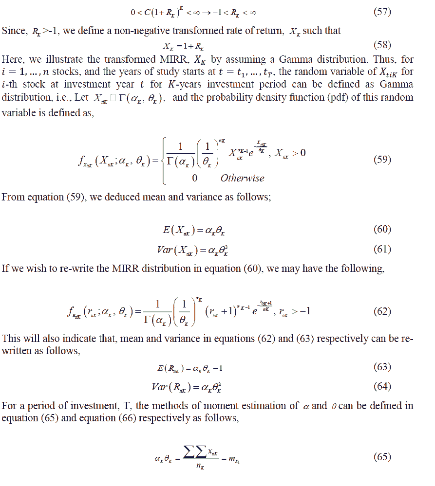
This study gives a further explanation of how to obtain the modified internal rate of return (MIRR) that is influenced by all the financial factors mentioned in the previous studies but also adds the treasury share dividends to the calculation, which has a huge impact on the investment’s rate of return. Also, the study proposes the transformed modified internal rate of return (MIRR) by adding the value of 1 to it to avoid any negative return since the return computed on any investment appears to be greater than –1.

As the rate of return can be in the form of a random variable, it will follow some statistical distribution. The normal distribution is the most popular for modelling the return in finance. For instance, (Sharpe, 1964; Thom, 1958) in explaining their theory of market equilibrium and Capital Asset Pricing Models, assumed that the return follows a normal distribution. But, in general, financial asset return distributions are not normal (Cont, 2001). Hence, other distributions should have been used alternatively (Fama, 1963). Gamma distribution is widely used in different scientific and technological fields, such as finance, meteorology, and networking studies (Kim, Lee & Sung, 2003; Kellison, 2009). Such a distribution is used to model positive continuous variables and it takes placelogicallyin the process where thewaiting timesbetween events are modelled the MIRR, which is also positive and continuous, instead of the traditional MIRR model proposed in (Sabri & Sarsour, 2019). Add to that the benefit of the information that we can score from the distribution’s statistical properties about the MIRR’s behaviour over different periods by assembling 62 Malaysian stocks from the property sector and determining whether the distribution of choice is a good fit to distribute the MIRR for long-term investment. We also use the distribution’s mean and variance to discuss the benefits of the long-term investment strategy. This paper further utilized the approach used by, Sabri & Sarsour (2019) in computing Modified Internal Rate Of Return (MIRR) for the property sector of Malaysian public listed companies for different investment periods.

To the best of the authors' knowledge, there is no recent approach that fit the modified internal rate of return on the assumption of Gamma distribution for property sector investment return. Therefore, the contributions of this study are presented as follows; (1) To introduce the modified internal rate of return model framework; (2) To fit the internal rate of return data set on the assumption of Gamma distribution; (3) To analyses the potential investment return of Malaysian property development sector for long term. The construction of the proposed approach would exhibit better analysis for successfully interpreting MIRR real-life datasets to detect profitable investment. This paper is organised as: in section 2, the materials and methods used in this study are presented and presented an example of how the MIRR is being computed extensively in Sabri & Sarsour (2019). Section 3 presented the Gamma distribution for modelling the MIRR. The Results and discussion have been reported in section 4. This study is conducted in Section 5.

Materials and Methods

Gamma Distribution Model

The gamma distribution is another widely used distribution. Its importance is largely due to its relation to exponential and normal distributions. The gamma function, shown by Γ(x), is an extension of the factorial function to real (and complex) numbers. Specifically, if n ∈{1,2,3,...}, then

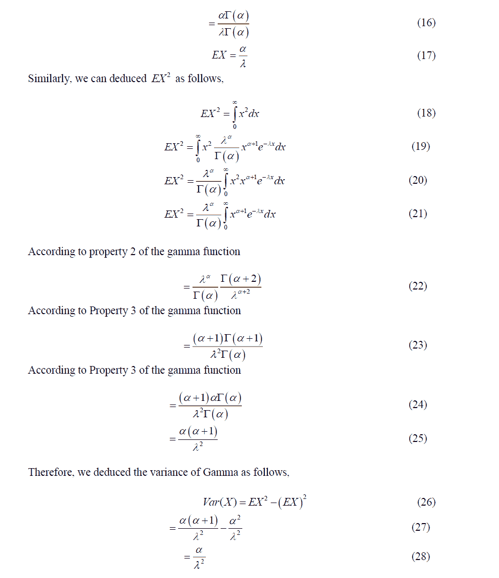
More generally, for any positive real number α, Γ(α) is defined as

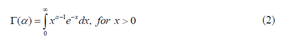
Figure 1 shows the gamma function for positive real values.

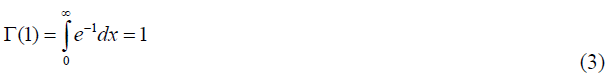
Note that for α=1, we can write

Using the change of variable x=λy, we can show the following equation that is often useful when working with the gamma distribution. Also, using integration by parts it can be shown that

Note that if α=n, where n is a positive integer, the above equation reduces to

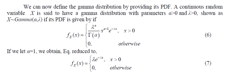
Thus, we conclude Gamma(1,λ)=Exponential(λ). More generally, if you sum n independent Exponential(λ) random variables, then you will get a Gamma(n,λ) random variable. We will prove this later on using the moment generating function. The gamma distribution is also related to the normal distribution as will be discussed later. Figure 2 shows the PDF of the gamma distribution for several values of α.

Using the properties of the gamma function, show that the gamma PDF integrates to 1, i.e., show that for α,λ>0, we have,

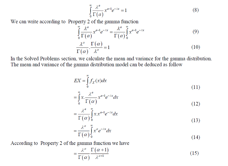
According to Property 3 of the gamma function

Modified Internal Rate of the Return Modelling Framework

In this paper, we study the public listed companies of the Malaysian property sector from the year 2008 to 2019. We chose one sector for simplicity to show a long-term investment strategy by gathering all companies’ return information. We started in 2008 as some companies did not provide an annual report for the previous year. We ended the data sample in 2019 to avoid the impact of Covid-19 on the market. The list of Malaysian public listed companies (Shariah compliance) is twice-yearly updated and can be downloaded from the Security Commission Malaysia website (www.sc.com.my). The updated list consists of the names of companies with their respective stock codes and is divided into several sectors, such as consumer products, industrial and property, to name a few. From this information, we can then download the annual reports that can be obtained from the Bursa Malaysia website (www.bursamalaysia.com) and the stock prices are accessible from The Wall Street Journal website (www.wsj.com).

For more information, the companies’ names can be referred to from the lists of the Shariah compliance website (www.sc.com.my). The bracket indicates the number of yearly dividends that the companies have declared over 12 years. In determining the companies’ MIRR, we need to extract the companies’ information such as dividend rates declared (in MYR) as well as the stock issuances that are usually announced every year in their annual reports. In addition, we also presented the events of share issuances over 12 years of duration that are presented in Table 2, reflecting’s the accumulation of the share units. The share accumulation function in this paper is denoted as . For instance, if there is no share issuance announced for a particular year, the share accumulation function (i.e. ) equals one. The share split from one (1) ordinary share to two (2) shares means the current share units earned will be multiplied by two units at the end of the year. The stock price here is reduced by half to enhance the liquidity of the share capital traded in the market. Hence, the company’s asset share remains unchanged. On the other hand, the bonus issue of one (1) share by two (2) existing ordinary shares indicates the company awards half of the share units that consequently accumulates to 1.5 share units at the end of the year. Some companies issue treasury shares which buy back the shareholders’ shares at random for a certain rate of the share price. Here, as our main objective is to accumulate our wealth by growing our share units and capital, we ignore this exercise by denying an offer to sell shares back to the company. In practice, most dividends are distributed in cash that is credited to the shareholders’ bank accounts. Some companies practice mandatory treasury shares by distributing cash dividends instead. That can be called a treasury share dividend. Here, the shareholder gets a dividend in cash, but his share units are reduced to a certain portion that is reported in the company’s annual reports. For further examples, please refer to stock codes 3417, 8494, 1538, and 5401. The detail of the computation of share accumulation is presented (Sabri & Sarsour, 2019).

Long Term Investment Framework

Sabri & Sarsour (2019) have underlined a long-term investment framework to increase the investor’s ownership of a certain company in a determined period of investment. By this strategy, the investor is committed to allocating his annual amount in advance to earn the share units of the company. His share capital will also be increased by reinvesting the annual dividends declared by the company. If the company that is held consistently makes a profit, it will generously award a share bonus that consequently increases the ownership of the investor. By utilizing this investment strategy, let a long-term investment model be as follows:-

a. An investor wishes to contribute his capital to stock, particularly an amount of annually in advanced mode.

b. If the company declares an annual dividend at -the year to the investor, he reinvests it together with annually in the same stock for the next year.

c. No withdrawals have been made during the investment period.

d. At the end of the year, the investor sells all his shares of the stock. The fund at the end of years is called the terminal fund and is denoted as .

There might be a case where the stock price for a particular company is too expensive or the amount of annual contribution might be too small. This will consequently result in an insufficient number of investors purchasing the stock in that kth year. Therefore, an investor wishes to allocate a sufficient amount at the beginning of (k+1)th the year. Here, we denote C^*_k = 0 and C^*_k+1 = 2C. From the above long term investment model, Figure 3 shows the cash flow of the investment underlined as follows:

Figure 3 indicates the series of cash out, C^*_k is used to invest in the stock and the amount of cash in, F(K) at the end of K the years. Mathematically, C^*_k can be set to either zero, a unit of C , or a product of an integer a_k with C, subject to the following,

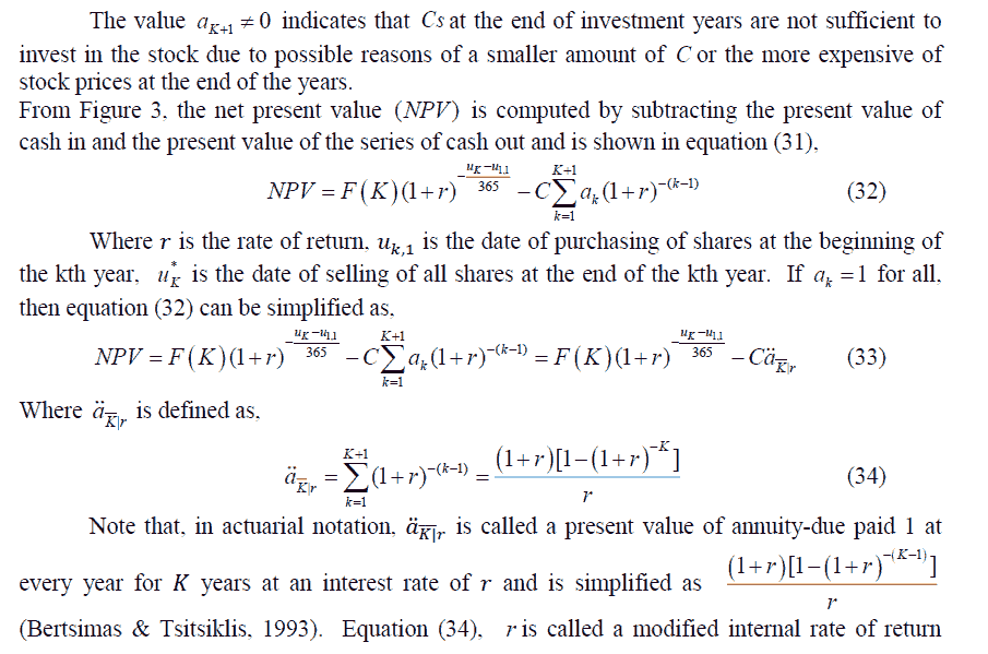
(MIRR) if NPV = 0 For example, let the information on this investing model be given as follows:

C =10,000MYR

Investment begins date (u_1,1) = 1^st January 2008

Investment end date, ( u^*_K) = 31st December 2019

The terminal fund F(12) =1,000,000MYR

Thus, r can be found by constructing equation (31) as follows,

By setting NPV = 0 , software computation assistance such as MS Excel is required. Initially, we set the initial value, r = -0.9 . The “Goal Seek” function is utilized by setting NPV = 0 to find the optimum value of r , that is then called as MIRR. For the above example, r = 0.3046 .

Stock Investment Cash flow

Let a discrete yearly time series be defined as, k =1,2...,K where K is an investment year period. We may also define u_k,₁ and u_k,2 as the respective dates in kth year, which are the date of purchase of share units made at the beginning and the date of the financial year report released. Here, we also note that, u_k,1< u_k,2< u_k+1,1 . Finally, we define the date where all share units are sold at the end of K the year, as u_k^*. At the beginning of kth year, an amount C was initially allocated to purchase E_k share units. Bursa Malaysia regulates investors to trade stocks on board lots. This means the investor is entitled to buy or sell his stocks in a number of lots only, where 1-lot of stock according to the Bursa Malaysia rules is determined to be equivalent to 100 share units. Hence, by assuming zero charges for brokerage fees, the share units bought, E_k and the exact contribution, C_k are defined as,

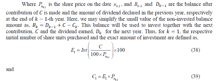
Finally, the cash balance for the first year is

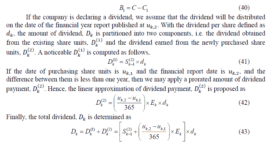
Figure 4 portrays the cash flow of the stock investment consisting of how the contributions and the cash dividends paid are used to purchase the share units.

From Figure 4, the investor allocates C₁ (<C) to purchase share units. The balance of the non-invested capital is denoted by (i.e., C-C₁equals to ). In the first year, the investor earns a dividend, D₁. This amount will be used together with B₁and new to purchase another share units, at the beginning of next year. The series of purchasing share units occurs recursively and lasts until the beginning of -th year. Since the dividend, is paid after the final payment, this dividend is not re-invested.

Accumulation of Share Modelling Framework

Share accumulation can be said as how the share units grow or turn down within one year based on the issuance of the shares. Therefore, we need to determine the share units before and after the share issuance events for a particular year. Here, we define S⁽¹⁾ as the share units before the share issuance event and S⁽²⁾ as the share units after the event. The relationship between these share units is explained by a so-called share issuance function, which is denoted as , and is generally presented as follows,

In this computation, we only consider the share issuances as follows:-

a. Share split (or sometimes called subdivision) or share consolidation. The share split issue means the shares are divided at a certain rate that is greater than 1. For example, the share is split from one (1) share into two (2) share units. Meanwhile, share consolidation means combining share issuance at a certain rate, which is a positive value and less than 1.

b. Bonus issue. The bonus issue is defined as additional share units awarded by the company to its shareholders generously for the consistent business performance of the company over the years.

c. Treasury share dividend. Some companies might not be able to pay the dividend in cash, but alternatively, distribute their repurchased shares to their members. This may increase a small fractional share to the shareholders, which is called a treasury share dividend.

By these underlined issues, the computation of the share accumulation function, g consists of share split (Spl), bonus share (Bns) and treasury share dividend (Tre) issues. Hence, the share accumulation function, g at k-th year is computed as follows,

Next, by utilizing equation (5), the accumulated share units at the end of k-th year is computed as,

And S_k⁽¹⁾ computed in equation (47) at the beginning of the first year, the shareholders' purchases E₁ share units.

The share units before the share issuance event are denoted as S_k⁽¹⁾ = E_k. Since he started investing in this stock, his share accumulation has grown to

At the end of the first year. He then purchases another E₂ share units for the next year, resulting to equation (49) at the beginning of the second year.

His share accumulation after the share issuance according to equation (50) at the end of the second year.

The procedure is repeated recursively by utilizing equation (50). This computation requires software assistance to compute the accumulated share units at the end of K investment years, S_k⁽²⁾ . Figure 5 illustrates the accumulation of the share units over four years.

In Figure 5, the shareholder purchases share units. The share units at the beginning of the year are denoted as . There was no share issuance announced in the first year. As the share units do not grow at the end of the first year, then,. In the second year, the share units are then arisen by purchasing another share units at the beginning. The share units at the beginning of the year are then denoted as . There is a share issuance that results in the growth of the share units at the rate of . Then, , where . In the third year, the share units are then arisen by purchasing the next share units at the beginning. The share units at the beginning are then denoted as . The share consolidation issue was announced to raise the share price. The share units are reduced at the end of the year at a rate of . Then, , where . Finally, in the fourth year, the share units are then arisen by purchasing another share units at the beginning. The share units at the beginning are then denoted as .

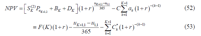
Sabri & Sarsour (2019) demonstrated the computation of g mathematically which consists of bonus issue and share split (or share consolidation) that can be referred to in equation (4). For the remaining stocks that do not experience these issuances, then g=1. The accumulated share units at the end of K-th year is denoted as S_k⁽²⁾. According to this investment framework, this volume of share units is going to be sold at the date of u^*_K. From Figure 2, the small balance of the non-invested amount, B_K together with the final dividend D_K are left in the shareholders’ cash. By selling all share units, the shareholder earns F(K), and thus, the terminal fund at the end of K-th year, is determined to be,

From Figure 1, the net present value of this investment framework by using discounted cash flow as in equation (31) can be generalized as follows,

If we wish to hold the stock of the company chosen for a long term period, the MIRR can be computed by constructing the stock investment projection first. Figure 1 indicates the stock investment projection as underlined above.

Sample Illustration

In this section, as an example and for simplicity, we implement the investment framework as introduced in section 2.2, by allocating MYR10,000 every beginning of the year for eight years investment period from the date of 3^rd January 2011 to the date of 3^rd January 2018 and withdrawing all our investment funds on the date of 31^st December 2018. We illustrate this investment projection by purchasing stock of Tropicana Corporation Berhad (Trop). By holding Trop company shares, which was formerly known as Dijaya Corporation Berhad (Dijacor) with the stock code 5401, we compute the MIRR from year 2011 to 2018. The company has been committed to distributing share dividends for all years. Furthermore, it also implemented a treasury share dividend in years 2015 and 2017 that reflected the increment of 0.013 and 0.012 portion of share units. Table 4 presents the share prices, dividend rates, and share issuance functions of Trop stock. Meanwhile, Table 1 and 2 indicates the cash flow and accumulated share units when purchasing this stock by this investment framework.

Table 1 Dividend, Share Price and Share Issuance of Tropicana Corporation Berhad
k	Date		(MYR)			Unit
	uK,1	uK,2	puK,1	pu*1	dK	SplK	BnsK	TreK	gK
1	1/1/11	31/12/11	0.910	1.219	0.0375	1	0	0	1
2	1/1/12	31/12/12	1.219	0.975	0.0225	1	0	0	1
3	1/1/13	31/12/13	0.975	1.155	0.0818	1	0	0	1
4	1/1/14	31/12/14	1.155	1.004	0.0400	1	0	0	1
5	1/1/15	31/12/15	1.004	0.959	0.0500	1	0	0.013	1.013
6	1/1/16	31/12/16	0.959	0.959	0.0450	1	0	0	1
7	1/1/17	31/12/17	0.959	0.888	0.0200	1	0	0.012	1.012
8	1/1/18	31/12/18	0.888	0.864	0.0160	1	0	0	1

Table 2 The Cash Flow of Investing of Trop Stock From Year 2011 to 2018
k	CK(MYR)	EK(Units)	BK(MYR)	Sk(1)(Units)	Sk(2)(Units)	DK(MYR)	Ck*(MYR)
1	9,919.00	10,900	81.00	10,800	10,900	407.63	10,000
2	10,483.40	8,600	5.23	19,500	19,500	438.75	10,000
3	10,432.50	10,700	11.48	30,200	30,200	2,466.45	10,000
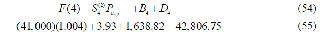
4	12,474.00	10,800	3.93	41,000	41,000	1,638.82	10,000
5	11,546.00	11,500	96.75	52,500	53,183	2,623.42	10,000
6	12,658.80	13,200	61.37	66,383	66,383	2,987.21	10,000
7	13,042.40	13,600	6.19	79,983	80,942	1,598.90	10,000
8	11,544.00	13,000	61.09	93,942	93,942	1,502.51	10,000

From Table 1 and 2, we may then compute the respective terminal investment, F(K) and MIRR=r_K by setting our investment period, K(i.e., K = 1,2,..,8). For example, if K = 4, then

From equation (53), by setting zero-valued of NPV, we may search for the, r₄, from the following equation,

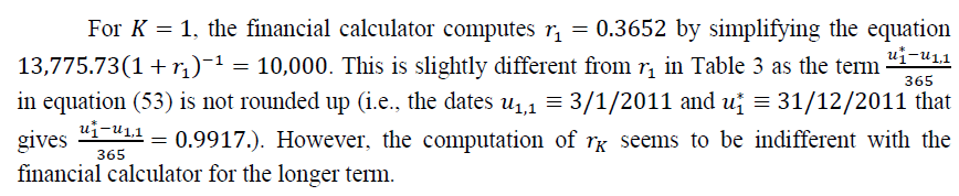
This results in . For further information, Table 6 indicates terminal investment and MIRR respectively based on investment periods from one to eight years, by contributing MYR10,000 every year starting from the year 2011. Table 3 reported the Terminal investment and MIRR of Trop Stock from the year 2011 to 2018.

Table 3 Terminal Investment and Mirr of Trop Stock From The Year 2011 To 2018
K	F(K)(MYR)	(MIRR) = rK	K	F(K)(MYR)	rK
1	13,775.73	0.3788	5	53,722.19	0.0240
2	19,456.48	-0.0182	6	66,709.40	0.0303
3	37,358.93	0.1138	7	73,481.85	0.0121
4	42,806.75	0.0273	8	82,729.74	0.0074

Gamma Modelling On the Modified Internal Rate of Return for the Property Sector

For i = 1,..,n stocks, and the years of investment starts at t = t₁,...,t_r the random variable of MIRR for i-th stock at investment year t for k-years investment period, can be denoted as R_tik where . It is very important to choose the best potential stocks to hold for a long term period. Furthermore, holding a stock for K year’s period may vary in terms of MIRR. Some might choose the best point of time to start investing, but it is very difficult to identify as the MIRR measure can only be observed yearly. Therefore, by assuming the MIRR for all companies and the starting time to invest are common, we may define the MIRR, denoted as R_tik, as a random variable having a mean and variance E(R_K) and Var(R_K) respectively.

In stock investment, we may either obtain profit (or total invested fund be greater than our total contributed investment) or lose everything. This indicates that even though we have been allocating an amount of C for every year, the terminal fund may either grow more than our total contributions or go to zero value. Let us consider investing a single amount of C at the beginning. For some time K, our terminal investment, is between 0 to infinite. Hence,

Results and Discussion

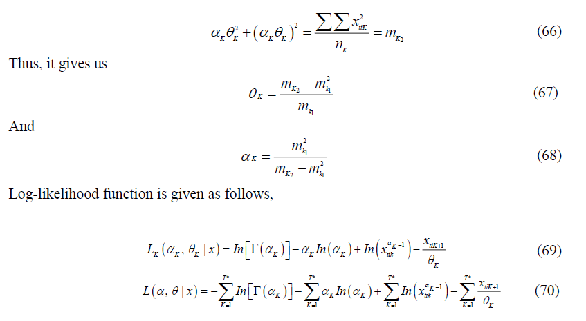
About 62 companies in the property sector were observed in our study. Here, we only develop the random variable of transformed MIRR from one to eight investment year periods (i.e., K = 1,...,8) as developing higher periods may not provide big enough data samples to work with. As the period of our study starts from the year 2008 and lasts until 2019, we may set t₁ = 2008 and t_T = 2009 and hence, T = 12. Furthermore, all companies’ MIRR is counted in our study. For example, for a one year investment period (i.e. K = 1) so the investor could invest in any given year from the 12 years then we manage to obtain a maximum of T = 12 multiplied with 62 companies and resulting in the sample size of 744, and if the investor invests at any given 8 years from the 12 years then for K = 8, we manage to get 310 sample size of MIRR. Table 4 summarizes the parameters estimates of the Gamma distribution as in equation (59) towards the transformed MIRR by using methods of moments over eight periods of investment of property sector in Malaysia.

Table 4 Parameters Estimates of Transformed Mirr By The Assumption of Gammadistributions
k	1	2	3	4	5	6	7	8
nk	744	682	620	558	496	434	372	310
m1k	1.155	1.135	1.124	1.114	1.110	1.111	1.102	1.090
m2k	1.907	1.452	1.359	1.306	1.284	1.276	1.246	1.215
αk	2.324	7.861	13.188	18.669	23.687	29.159	36.620	43.740
θk	0.497	0.144	0.085	0.060	0.047	0.038	0.030	0.025
E(Xk)	1.155	1.135	1.124	1.114	1.110	1.111	1.102	1.090
E(Rk)	0.155	0.135	0.124	0.114	0.110	0.111	0.102	0.090
Var(Xk)	0.574	0.164	0.096	0.066	0.052	0.042	0.033	0.027
KS	0.191*	0.103*	0.079*	0.073*	0.056	0.041	0.049	0.066

In this study we considered 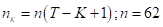. Furthermore, KS indicate the Kolmogorov-Smirnov test. Figure 3 illustrates the PP-Plot of Gamma distribution against the empirical distribution of X. F(Gamma) Indicates the cumulative distribution function (cdf) value Gamma distribution, whereas F_n is the empirical cdf value among K investment periods from the year 2008 to 2019. KS from Table 4 indicates the Kolmogorov-Smirnov statistic for verifying whether the transformed MIRR for each investment period is being Gamma distributed. At 5%, the KS are being compared with the critical region of . Here, the KS rejects the null hypothesis of being Gamma distributed for the return at lower investment periods (i.e. from 1 to 4 years). Hence, the transformed MIRR is well fitted with Gamma distribution for a longer period of investment.

From Table 4, both the means and variances of transformed MIRR, as displayed in Figure 7, decline over the investment period. This means purchasing companies’ shares of the property sector is very attractive for a short-term period, but may have a high risk of committing it. This is consistent with the theorem stating that the greater the stock return, the larger the volatility (Markowitz, 1952). Meanwhile, we might be certain to hold the stock for a longer period as we have seen the decline in the variance of the MIRRs and a flattening 3-years investment duration onwards for this sector.

The contribution of this study to the literature can be written as follows:

1. The investment rate of return is affected by more than cash dividends. Other practices such as share issuance that come in several forms, such as share splits, bonus issues, or treasury share dividends, have an impact on the rate of return. Therefore, it is important to have a fair calculation for share issuance, as shown by the share accumulation function in equation (45), to get a realistic picture of MIRR.

2. As the return from any investment can be a positive value or zero but never a negative value, we transformed the MIRR by adding 1 to it before we distributed it using a gamma distribution.

3. The assumption that MIRR is common for all points of investment’s beginning time allows us to start investing at any time regardless of current economic situations, as we are only concerned with the period of investment in this However, the issue of considering the right time to invest should be addressed as the current MIRR might be auto-correlated with the previous time.

4. Continuous and positive distributions such as gamma distribution, are efficient tools to model the MIRR for long term investment. The distribution properties and the KS test of the MIRR support the long-term investment strategy as shown in the result.

5. This paper offers a long-term investment model based on comprehensive MIRR competition for 26 companies of the Malaysian property sector, such a model is useful for helping organizations (governmental or not) or individuals to make wise investment decisions. It also applies to other sectors of the Malaysian or the international stock market.

Conclusion

An exhaustive computation of MIRRs for all stocks from various investment durations of the property sector supports that the MIRR exhibits more than –1, thus requiring the transformation distribution into the non-negative form. After transforming is made, the Gamma distribution is suggested in this paper and the statistical properties of this distribution have been presented. To make it easier to compute the parameters, the method of the moment is utilized. To test the adequacy of the model fitted, Kolmogorov-Smirnov was used. The Gamma distribution is well fitted to the transformed MIRR for a longer investment period. Furthermore, the variance of the transformed MIRR for a longer period is decreasing, thus indicating that investing in company stocks for a longer term is less risky and this suggests we hold them longer, as being practised by many fund managers, such as employee provident funds as well as unit trust funds. Maximum likelihood is a beneficial tool to estimate Gamma distribution parameters. However, it is a tedious process as differentiating its log-likelihood function towards forms a non-linear function, and thus the estimated value of can not be determined easily. Metaheuristics algorithms such as simulated annealing (Abbasi, Jahromi, Arkat & Hosseinkouchack, 2006; Abubakar & Sabri, 2021; Abubakar & Sabri, 2021) can be used towards such exponential family distributions as has been developed by Biondi (2006); Baldwin (1959). Here, they estimated the Weibull distribution parameters by using this algorithm.

References

References

Ahmad, A.G. (2015). Comparative study of bisection and newton-rhapson methods of root finding problems. International Journal of Mathematics Trend and Technology, 19(2), 121–129.

GoogleScholar, Indexed at

Abubakar, H., & Sabri, S.R.M. (2021). Incorporating simulated annealing algorithm in the Weibull distribution for valuation of investment return of Malaysian property development sector. International Journal for Simulation and Multidisciplinary Design Optimization, 12, 22.

Crossref, GoogleScholar, Indexed at

Abubakar, H., & Sabri, S.R.M. (2021). A simulation study on modified weibull distribution for of investment return. Pertanika J. Sci. & Technol, 29(4), 2767 – 2790.

Crossref, GoogleScholar, Indexed at

Abbasi, B., Jahromi, A.H.E., Arkat, J., & Hosseinkouchack, M. (2006). Estimating the parameters of Weibull distribution using Simulated Annealing algorithm. Applied Mathematics and Computation, 183, 85-93.

Crossref, GoogleScholar, Indexed at

Baldwin, R.H. (1959), How to assess investment proposals. Harvard Business Review, 37(3), 98-104.

Besley, S., & Brigham, E.F. (2015). CFIN4 (with Finance CourseMate). (4 Edition), Cram101 Textbook Reviews.

Bertsimas, D., & Tsitsiklis, J. (1993). Simulated annealing. Statistical Sciences, 8(1), 10-15.

Biondi, Y. (2006). The double emergence of the modified internal rate of return: The neglected financial work of Duvillard (1755-1832) in a comparative perspective. The European Journal of the History of Economic Thought, 13(3), 311-335.

Crossref, GoogleScholar, Indexed at

Bonazzi, G., & Lotti, M. (2016). Evaluation of investment in renovation to increase the quality of buildings: A specific Discounted Cash Flow (DCF) Approach of Appraisal. Sustainability, 8(268), 1-17.

Crossref, GoogleScholar, Indexed at

Brealey, R.A., Myers, S.C., & Allen, F., (2006). Principles of corporate finance (8th Edition). Boston: McGraw-Hill/Irwin.

Cont, R., (2001). Empirical properties of asset returns: Stylized facts and statistical issues. Quantitative Finance, 1, 1-14.

Crossref, GoogleScholar, Indexed at

Fama, E.F. (1963). Mandelbrot and the stable Paretian hypothesis. The Journal of Business, 36(4), 420-29.

GoogleScholar, Indexed at

Kellison, S.G. (2009). The theory of interest, (3^rd Edition). McGraw Hill Education.

Indexed at

Kim, S., Lee, J.Y., & Sung, D.K., (2003). A shifted gamma distribution model for long-range dependent internet traffic. IEEE Communications Letters, 7(3), 124-126.

Crossref, GoogleScholar, Indexed at

Kierulff, H., (2008). MIRR: A better measure. Business Horizons, 51(4), 321-329.

Crossref, GoogleScholar, Indexed at

Markowitz, H. (1952). Portfolio selection. The Journal of Finance, 7(1), 77-91.

Crossref

Pascual, N., Sison, A.M., Gerardo, B.D., & Medina, R. (2018). Calculating Internal Rate of Return (IRR) in Practice using Improved Newton-Raphson Algorithm, Philippine Computing Journal, 13(2), 17–21.

GoogleScholar, Indexed at

Queirós, S.M.D. (2005). On the emergence of a generalised gamma distribution. Application to traded volume in financial markets, Europhysics Letters, 71, 339-345.

Crossref, GoogleScholar, Indexed at

Ross, A.S., Westerfield, R.W., & Jordan, B.D. (2010). Fundamental of Corporate Finance. The McGraw-Hill Companies, Inc.

Satyasai, K.J.S., (2009). Application of modified internal rate of return method for watershed evaluation. Agricultural Economics Research Review, 22 (Conference Number), 401- 406.

GoogleScholar, Indexed at

Sabri, S.R.M., & Sarsour, W.M. (2019). Modelling on stock investment valuation for long-term strategy. Journal of Investment and Management, 8(3), 60-66.

Crossref, GoogleScholar, Indexed at

Sharpe, W.F., (1964). Capital asset prices: A theory of market equilibrium under conditions of risk. The Journal of Finance, 19, 425-442.

Crossref, GoogleScholar, Indexed at

Thom, H.C.S. (1958). A note on the gamma distribution. Monthly Weather Review, 86(4), 117-122.

Crossref, GoogleScholar, Indexed at

Received: 30-Nov-2021, Manuscript No. JMIDS-21-8770; Editor assigned: 02- Dec -2021, PreQC No. JMIDS-21-8770 (PQ); Reviewed: 11- Dec -2021, QC No. JMIDS-21-8770; Revised: 17-Dec-2021, Manuscript No. JMIDS-21-8770 (R); Published: 05-Jan-2022.