Research Article: 2022 Vol: 25 Issue: 2
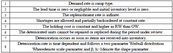
Two ware-houses fuzzy inventory model for deteriorating items with ramp type demand and shortages
Garima Sethi, Research Scholar, SRM Institute of Science and Technology, Delhi-NCR Campus
Ajay Singh Yadav, SRM Institute of Science and Technology, Delhi-NCR Campus
Chaman Singh, Acharya Narendra Dev College
Citation Information: Sethi, G., Yadav, A. S., & Singh, C. (2022). Two ware-houses fuzzy inventory model for deteriorating items with ramp type demand and shortages. Journal of Management Information and Decision Sciences, 25(2), 1-22.
Abstract
In this paper we developed a fuzzy inventory model for single spoilage two-parameter weibull-distribution degradation rate, ramp type demand, and partial backordering at a constant rate. In the current market scenario, an increase in the cost of the inverter affecting the total cost of inventory costs due to inflation can increase at any time of the order length.The increase in the cost of the components of the inventory cannot be pre-determined due to the uncertainty of the market situation. Therefore, we have considered the interval based fuzzy concept to handle the uncertainty condition. Ordering cost, the cost of holding in both ware-houses is considered a triangular fuzzy number.
Keywords
Weibull deterioration distribution; Partial backlogging; Rramp type demand; Fuzzy holding cost; Ordering cost.
Introduction
In traditional models, many researchers have considered the rate of demand to be constant, linear time dependent, stock dependent or accelerating over time and the same trend of considering this type of demand still continues but it is not always true that demand occurs in the same pattern. The assumption of a constant demand rate is generally valid in the mature phase of a product's life cycle. Several models have developed inventory models for items stored in two ware-houses under modelling assumptions. The rate of demand in these models is assumed to be constant over time. However, in practice a person will accept the demand for separation over time.Most classical inventory models assumed that the utility of the inventory remains constant during the period of their storage. But in real life, degradation occurs during the storage period. The deterioration of physical objects is a common phenomenon in the real world that can occur for various reasons and has attracted a lot of attention from various researchers.In recent years, the problem of inventory worsening has received considerable attention. Most products such as medicine, blood, fish, alcohol, gasoline, vegetables, and radioactive chemicals have self-life, and once spoiled they begin to deteriorate. The listed researchers, above, have taken care of deteriorating objects in their models and have developed models accordingly. In addition to inventory deterioration, limited storage is also a major practical problem for real life.Due to lack of large storage space at important market places, one should be forced to own a small ware-house at important market places. At times, it may be profitable for the retailer to order quantities in excess of its own warehouse capacity. In this situation retailers require additional space to store bulk purchased items and therefore prefer to rent the house for a limited period. A specially equipped storage facility is required to reduce the amount of spoilage. The cost of building such a storage facility for a limited period is usually excessive. Therefore, it may be difficult for a retailer to have such a storage facility of its own at retail outlets. To handle this situation, another storage space is required, making the necessary facilities available. To launch some new products e.g. Fashionable items, clothing, electronic items, mobiles etc. The uncertainty of change in any component of an inventory model can occur and cannot be determined in advance until we arrive at that position or time.For example increasing prices, affecting total inventory costs or demand, shortages, etc. It is not easy to estimate how much? and/or when increases / decreases in components of an inventory model occur for the foreseeable future? One of management's most concerns is to decide when and how much to order so that the costs associated with the inventory system are minimized.This is more important when some or more products in the inventory are deteriorating. These types of situations can be dealt with the help of fuzzy based concepts such as fuzzy set theory, fuzzy numbers, etc., which were introduced by Zadeh (1965) in their paper, followed by many using fuzzy set theory in fuzzy environments. Papers have been developed. Zaidh (1965) considered an inventory model when making decisions in fuzzy environments. Jain (1976) developed a fuzzy inventory model when making decisions in the presence of fuzzy variables. DuBois and Prade (1978) defined some operations on fuzzy numbers. In general, demand is assumed to be either constant or increasing over time (Kumar et al., 2007). An economic production volume is developed with fuzzy demand and rate of decline. Syed and Aziz (2007) consider a signed distance method for a fuzzy inventory model without drawbacks. De and Rawat (2001) developed a fuzzy inventory model without reduction using triangular fuzzy number. Jaggi et al. (2012) developed a fuzzy inventory model for deteriorating goods over time demand and scarcity. Datta and Kumar (2012) considered an optimal replenishment policy for an inventory model without reduction by assuming fajita in demand. Halim et al. (2008) developed a fuzzy inventory model for perishable goods with stochastic demand, partial backlogging, and fuzzy deterioration rates. Gani and Maheshwari (2010) discussed the retailer's order policy under two levels of payment delays and considered the demand and selling price as a triangular fuzzy number. He used the Graded Mean Integration Representation Method for the differentiation. Halim et al. (2010) addressed a very sizing problem with stochastic machine breakdown and fuzzy repair time using the signed distance method in an unreliable production system.Singh and Singh (2008) developed a fuzzy inventory model for the finite rate of replenishment using the signed distance method. Jaggie et al. (2018a) discussed a decrease in trade with inventory quality deteriorating commodities and partially backlogged short lived shortages for thoughtful decision making. Jaggi et al. (2018b) discussed the tau-warehouse inventory model for non-instantaneous perishable items under various dispatch policies. Khanna et al. (2017) detailed about inventory modelling for incomplete quality items with price dependent demand and short backorder sales under credit financing. Jaggi et al. (2018c) differentially defined criteria for poor quality items with increasing demand and partial backlogging. Khanna et al. (2016) defined credit for deterioration of goods of imperfect quality with acceptable quality. Jaggi et al. (2015) discussed an inventory model for deteriorating goods with ramp type demand under trapped environment. Yadav et al. (2020) studied supply chain management and its impact of industrial development on the defined electronic components warehouse. Yadav and Swamy (2018a;b; 2019a;b) discussed about an inventory model for non-instantaneously deteriorating commodities with variable holding costs under two-storage and a volume flexible two-warehouse model with volume fluctuations and Holding costs with inflation and a partial backlog production. Inventory lot-size model with time-varying hold and time-varying cost and Weibull decline and supply chain model for items deteriorating with linear stock dependent demand under the Impression and Inflationary Environment (Pandey et al., 2019; Yadav et al., 2017a;b;c) It is discussed that with the chain inventory model, warehouse and distribution centers for perishable goods and supply centers for the deteriorating goods and warehouses for the chemical industry supply chain, With distribution centers using the artificial BE colony algorithm. Influence of inflation on the two-warehouse inventory model for commodities deteriorating over time and demand and two storage systems for two warehouses with soft computing optimization and an inflationary inventory model for deterioration of items under the supply chain inventory model.
In literature, own warehouses are abbreviated as OWs, and rented warehouses as RWs, and it is generally assumed that rent warehouses compare to own warehouses Has better storage facilities available and because of this, the rate decline is smaller than OW resulting in higher holding costs on RW, so retailers prefer to consume goods from RW and then OW first.Inspired by the above papers, we developed a two-ware-house inventory model for the demand rate as a general ramp-type function of time and studied the effect of the two-parameter Weibull distribution degradation rate and fajita with fuzzy triangular numbers.Both the ordering cost and the holding costin ware-house are treated as fuzzy triangular numbers and the signed distance method is used to defreeze the total inventory cost. Only one item is included in this study.Shortage is allowed and partially backordered at a constant rate and the results of crisp and fuzzy models are compared with the help of numerical examples. Sensitivity is also played for both model son limiting parameters.
Assumption and Notations
Assumptions
The following assumptions were used in this research (Table 1)
| TABLE 1 Crisp Model |
||||||
|---|---|---|---|---|---|---|
| Case |  |
 |
 |
 |
 |
 |
| Example 1 | ||||||
| 1 | 0.3227 | 7.2985 | 21.3194 | 28.9545 | 34 | 194.88 |
| 2 | 0.5302 | 7.6269 | 29.5440 | 37.7011 | 35 | 267.05 |
| 3 | 0.5178 | 1.4836 | 04.9466 | 6.948 | 34 | 213.85 |
| Example 2 | ||||||
| Case | |
|
|
|
|
|
| 1 | 0.8341 | 6.8149 | 08.7521 | 16.4011 | 182 | 2356.53 |
| 2 | 0.2106 | 7.0602 | 09.3465 | 16.6173 | 028 | 2087.43 |
| 3 | 0.4845 | 1.0090 | 0.8298 | 02.3233 | 084 | 1012.20 |
Notation
The following notation is used throughout the paper:
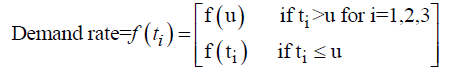
W =Capacity of OW α =Scale parameter of the deterioration rate in OW and 0<α<1 α =Scale parameter of the deterioration rate in OW and 0<α<1 g=Scale parameter of the deterioration rate in RW,α> g h=Shape parameter of the deterioration rate in RW and h>1. β =Shape parameter of the deterioration rate in OW and β>1. fd=Fraction of the demand backordered during the stock out period C0=Ordering cost per order Dc=Deterioration cost per unit of deteriorated item in RW and OW Hw=Holding cost per unit per unit time in OW Hr=Holding cost per unit per unit time in RWsuch that (hr-ho)>0 Sc=Backlogging cost per unit per unit time Lc=Opportunity cost for lost sales per unit Qmax,i=Maximum order quantity at the end of cycle length for i=1,2,3 T1=Time with positive inventory in RW T1+T2=Time with positive inventory in OW T3=Time when shortage occurs in OW T=Length of the cycle i.e.T=T1+T2+T3 Ii jt (ti )=Inventorylevelforthesystemattimetisuchthat0?ti?Tiandforcasesi=1,2,3 Rti =Inventory level in RW at time ti=0 for cases i= 1, 2, 3 φti =Inventory cost per cycle for cases i=1,2,3 φ t=Optimal inventory cost per cycle per unit of time The rate of deterioration is given as follows: t i=Time to deterioration, ti >0 Instantaneous rate of deterioration in OW 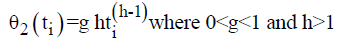 {~ Sign represent the fuzziness of the parameters}
Mathematical Model
Crisp Model Case-1: 
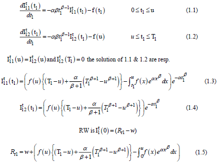
Therefore the inventory level is governed by the following differential equations
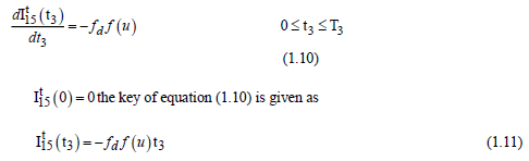
Inventory level time interval (0 T1) in OW due to malfunction only until the inventory reaches zero on RW.
Both warehouses are empty during the time interval (0 T3) at T3 = 0.
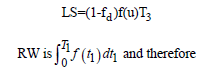
The lost sales volume of inventory throughout the shortage time is
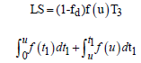
Therefore the amount of inventory that has been spoiled during this period is
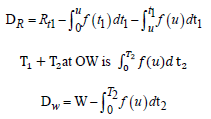
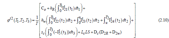
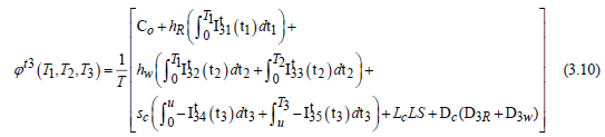
The total applicable inventory cost per unit of time
Case-2: 

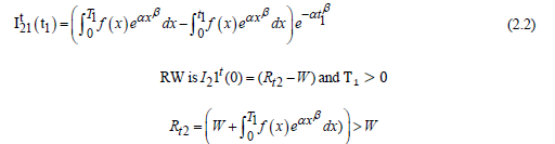
 The solution of equation 2.1 is
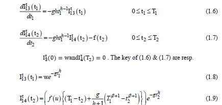
Applying the same logic as OW to the time intervals (0 T1) and (0 T2), the following differential equations are obtained
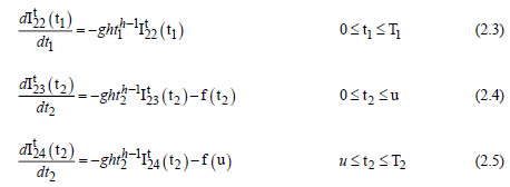
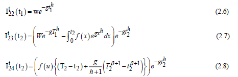
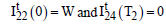 the solution of (2.3), (2.4) & (2.5 are respectively
Furthermore, both warehouses are empty during the time interval (0 T3) at T3 = 0, and a portion of the shortfall is returned to the next “replenishment” and is similar to Equation (1.10) of Case-1

The lost sales volume of inventory throughout the shortage period is
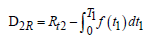
RW is the amount of inventory deteriorating
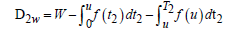
The total demand during time epoch 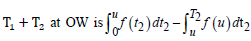 and amount of inventory deteriorated during the period
 at OW is
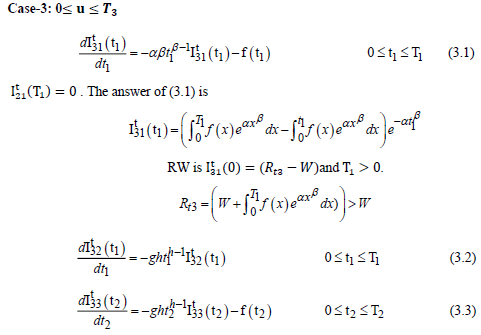
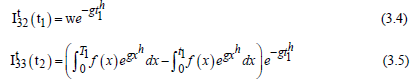
With boundary conditions 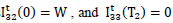 , the solution of (3.2)& (3.3) are respectively.
Furthermore, both warehouses are empty during the time interval (0 T3) at T3 = 0,
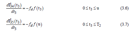
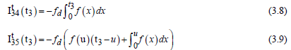
With boundary conditions  , the answer of (3.6) & (3.7) are respectively
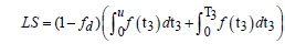
The lost sales volume of inventory during the shortage period is
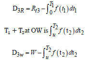
RW is  and therefore
RW is the amount of inventory deteriorating
Fuzzy Model
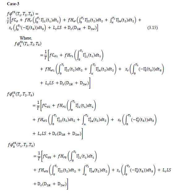
The model developed above is a crisp mock-up in which all criteria are set but this is not always possible. In the current global market, the value of parameters such as cost, demand can fluctuate due to inflation and uncertainty of any reason (eg low production, natural hazards, etc.) and it can fluctuate around its own value. . The fluctuations at any time cannot be predetermined until we reach the state of that time.Therefore, the only possibility is to consider the possible range of fluctuations. To deal with this type of uncertain condition, we developed a fuzzy model looking at the ambiguity of some parameters affecting the total inventory cost. We have taken the order cost and the investment cost as fuzzy numbers in both warehouses represented by a triangular number.The model is solved using the signed distance method to reduce the total inventory cost. The results from three different cases are compared with the value of the crisp model. Fazimodel for three different cases is as follows:
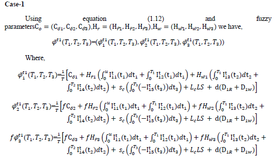
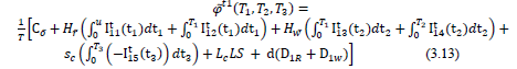
Thus with above fuzzy parameters the total inventory cost in case-1 is given by the eq.
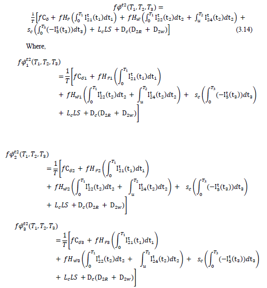
Similarly for other two cases using above defined fuzzy parameters the total inventory cost is given by following equations
Case-2
Sensitivity Analysis
Sensitivity analysis is performed on parameter values of example-1.
Crisp Model
From Table 1 and Table 12, we see that serially the thin millthere value of the total pertinent inventory cost in one suitable unit for Case-1 compared to the other two cases in the model compared to the crisp model (more details refer to Appendix).
From each Table 2, it is observed that in each case, the total inventory cost and the cycle length are directly proportional to the cost of ordering, i.e. the total inventory cost as well as cycle length with an increase in ordering; both increases.
| Table 2 Variation in total inventory cost with respect to  |
|||||||
|---|---|---|---|---|---|---|---|
| Case | |
|
|
|
|
|
|
| 1 | 200 | 0.2871 | 7.3084 | 20.1123 | 27.7078 | 21 | 184.29 |
| 500 | 0.3227 | 7.2985 | 21.3194 | 28.9406 | 34 | 194.88 | |
| 600 | 0.3342 | 7.3081 | 21.7101 | 29.3524 | 24 | 198.31 | |
| 2 | 200 | 0.5147 | 7.6329 | 28.6260 | 36.7736 | 33 | 258.99 |
| 500 | 0.5302 | 7.6269 | 29.5441 | 37.7012 | 35 | 267.05 | |
| 600 | 0.5315 | 7.6250 | 29.8452 | 38.0017 | 35 | 269.69 | |
| 3 | 200 | 0.4194 | 1.3625 | 03.8423 | 5.6242 | 24 | 166.14 |
| 500 | 0.5178 | 1.4836 | 04.9466 | 6.948 | 34 | 213.85 | |
| 600 | 0.5440 | 1.5177 | 05.2708 | 7.3325 | 36 | 227.85 | |
From each Table 3, it is observed that in each case the total inventory cost increases when the cost in RW decreases, the ordering length increases. When the cost increases in RW, both the total inventory cost and the length of the ordering cycle increase.
| Table 3 Variation In Total Inventory Cost With Respect To  |
|||||||
|---|---|---|---|---|---|---|---|
| Case | |
|
|
|
|
|
|
| 1 | 1 | 0.9340 | 7.2982 | 21.3720 | 29.6042 | 53 | 195.40 |
| 2 | 0.4827 | 7.2981 | 21.3742 | 29.155 | 31 | 195.34 | |
| 5 | 0.1921 | 7.2998 | 21.1724 | 28.6643 | 53 | 198.10 | |
| 2 | 1 | 0.9771 | 7.6279 | 29.4002 | 38.0052 | 94 | 265.79 |
| 2 | 0.6673 | 7.6272 | 29.4997 | 37.7942 | 50 | 266.66 | |
| 5 | 0.3928 | 7.6266 | 29.5887 | 37.6081 | 22 | 267.41 | |
| 3 | 1 | 0.9268 | 1.4693 | 5.1118 | 7.5079 | 86 | 208.04 |
| 2 | 0.6458 | 1.4755 | 4.9014 | 7.0227 | 48 | 211.88 | |
| 5 | 0.3872 | 1.4886 | 4.9937 | 6.8695 | 22 | 215.88 | |
From Table 4, it is observed that in each case the total inventory cost increases when the cost in OW decreases and the cycle length decreases. When the cost rises, the total inventory cost as well as the cycle length increase.
Fuzzy Model
| Table 4 Variation In Total Inventory Cost With Respect To  |
|||||||
|---|---|---|---|---|---|---|---|
| Case | |
|
|
|
|
|
|
| 1 | 1 | 0.2106 | 7.0602 | 9.3765 | 16.6437 | 9 | 199.40 |
| 3 | 0.4858 | 7.5578 | 32.4287 | 40.4723 | 31 | 340.78 | |
| 4 | 0.5053 | 7.4838 | 38.7984 | 46.7875 | 32 | 348.26 | |
| 2 | 1 | 0.4434 | 7.4828 | 19.1624 | 27.0886 | 27 | 175.95 |
| 3 | 0.5731 | 7.6808 | 37.6472 | 45.9011 | 39 | 338.15 | |
| 4 | 0.5957 | 7.7105 | 44.5261 | 52.8323 | 42 | 398.52 | |
| 3 | 1 | 0.5178 | 1.4836 | 4.9466 | 6.948 | 34 | 213.85 |
| 3 | 0.3670 | 0.8445 | 5.6263 | 6.8378 | 20 | 226.82 | |
| 4 | 0.2443 | 0.7251 | 5.7831 | 6.7525 | 12 | 249.97 | |
From Tables 5, 6 and 7, it is observed that in each case, the total inventory cost in the fuzzy model decreases when working with a single fuzzy parameter and with an increase in cycle length.
| Table 5 Variation In Total Inventory Cost With Respect To |
||||||
|---|---|---|---|---|---|---|
| Case |  |
 |
 |
 |
 |
 |
| 1 | 0.3342 | 7.2955 | 21.7104 | 29.3401 | 24 | 148.73 |
| 2 | 0.5302 | 7.6227 | 29.5441 | 37.697 | 35 | 202.28 |
| 3 | 0.4861 | 1.0656 | 5.7151 | 7.2668 | 31 | 185.28 |
| Table 6 Variation In Total Inventory Cost With Respect To |
||||||
|---|---|---|---|---|---|---|
| Case | |
|
|
|
|
|
| 1 | 0.3007 | 7.2956 | 21.6888 | 29.2851 | 22 | 148.18 |
| 2 | 0.5302 | 7.6227 | 29.5441 | 37.697 | 35 | 202.28 |
| 3 | 0.4861 | 1.0656 | 5.7151 | 7.2668 | 31 | 185.28 |
| Table 7 Variation In Total Inventory Cost With Respect To |
||||||
|---|---|---|---|---|---|---|
| Case | |
|
|
|
|
|
| 1 | 0.4963 | 7.4653 | 36.6172 | 44.5788 | 32 | 246.84 |
| 2 | 0.5898 | 7.7022 | 42.3366 | 50.6286 | 41 | 284.45 |
| 3 | 0.2902 | 0.7596 | 5.7376 | 6.7874 | 14 | 186.00 |
From each Table 8, it is observed that in each case, the total inventory cost decreases and the cycle length increases when working with cost and holding cost as fuzzy parameters in RW.
| Table 8 Variation In Total Inventory Cost With Respect To  |
||||||
|---|---|---|---|---|---|---|
| Case | |
|
|
|
|
|
| 1 | 0.3007 | 7.2956 | 21.6828 | 29.2791 | 22 | 148.18 |
| 2 | 0.5036 | 7.6249 | 29.8555 | 37.984 | 32 | 202.34 |
| 3 | 0.4570 | 1.0662 | 05.7237 | 7.2469 | 28 | 185.56 |
From Tables 9, 10 and 11 it is observed that in Cases-1 and Cases-2, the total inventory cost increases, while in OWs work with ordering cost and holding cost and as fuzzy parameters There is a combination of three costs and the total inventory in Case-3. Cost reduction but increasing cycle length in each case.
| Table 9 Variation In Total Inventory Cost With Respect To  |
||||||
|---|---|---|---|---|---|---|
| Case | |
|
|
|
|
|
| 1 | 0.4963 | 7.4653 | 36.6172 | 44.5788 | 32 | 246.84 |
| 2 | 0.5933 | 7.7014 | 42.5612 | 50.8559 | 42 | 300.66 |
| 3 | 0.3303 | 0.7776 | 06.0910 | 7.1989 | 17 | 196.75 |
| Table 10 Variation In Total Inventory Cost With Respect To  |
||||||
|---|---|---|---|---|---|---|
| Case | |
|
|
|
|
|
| 1 | 0.4400 | 7.4663 | 36.6172 | 44.5235 | 29 | 245.09 |
| 2 | 0.5548 | 7.7021 | 42.3466 | 50.6035 | 37 | 284.54 |
| 3 | 0.2722 | 0.7597 | 5.7401 | 6.772 | 13 | 186.09 |
| Table 11 Variation In Total Inventory Cost With Respect To  |
||||||
|---|---|---|---|---|---|---|
| Case | |
|
|
|
|
|
| 1 | 0.4468 | 7.4653 | 36.6080 | 44.5201 | 29 | 246.78 |
| 2 | 0.5558 | 7.7014 | 42.5713 | 50.8285 | 38 | 286.02 |
| 3 | 0.3105 | 0.7764 | 6.0724 | 7.1593 | 16 | 196.86 |
| Table 12 Fuzzy Model |
||||||||||
|---|---|---|---|---|---|---|---|---|---|---|
| Example 1 | ||||||||||
| Case | |
|
|
|
|
|
||||
| 1 | 0.3418 | 7.2933 | 21.9682 | 29.6033 | 24 | 150.43 | ||||
| 2 | 0.5385 | 7.6237 | 30.0446 | 38.2068 | 36 | 203.58 | ||||
| 3 | 0.5041 | 1.0800 | 05.9240 | 07.5441 | 32 | 192.05 | ||||
| Example 2 | ||||||||||
| Case | |
|
|
|
|
|
||||
| 1 | 0.8418 | 6.6785 | 8.8797 | 16.4000 | 186 | 1785.57 | ||||
| 2 | 0.8994 | 6.5832 | 8.0728 | 15.5554 | 212 | 1668.72 | ||||
| 3 | 0.4845 | 1.0090 | 0.8298 | 02.3233 | 084 | 0759.15 | ||||
For each case of crisp model and in Figure 1the graph shown in Figure 2 is for each case of the fuzzy model show that there is a point where the minimum cost with constraint in the inventory system is that T1, T2 and T3 are all positive.

Figure 1:Graphical Representation Of Convexity For Crisp Model.

Figure 2:Graphical Representation Of Convexity For Fuzzy Model.
Conclusion
A deterministic inventory mock-up is obtainable to settle on the most favourable inventory cost for the two-warehouse inventory mock-up with ramp type demand, Weibull distribution degradation rate and partial backlog at constant rate. Two models namely a crisp model and a fuzzy model have been developed and numerical examples have been presented to illustrate and validate themodels.The results are obtained and compare with the help of appropriate software. Sensitivityanalysis is performed on some chosen parameters. The fuzzy model is solved with the rescue of triangular fuzzy numbers with the help of the signed distance method.In addition, this model can be normalized by taking into account the price-dependent demand, stock-dependent demand, and a constant decline rate with other realistic combinations.
We residential a two-warehouse inventory mock-up for demand rate as a universal ramp-type function of moment and have studied the effect of the two-parameter Weibull distribution degradation rate and fajita with fuzzy triangular numbers.The cost of ordering and holding costs in both ware-houses are treated as fuzzy triangular numbers and the signed distance method is used to defile the total inventory cost. Only one item is included in this study. Shortages are authorized& partially backordered at a constant rate and the results of the crisp and fuzzy models are compared with the help of numerical examples. Sensitivity is also played for both model son limiting parameters.
References
Datta, D., & Kumar, P. (2012). Fuzzy Inventory Model without shortages by Using Trapezoidal Fuzzy Number with Sensitivity Analysis. IOSR Journal of Mathematics, 4, 32-37.
Gani, A. N., & Maheshwari, S. (2010). Supply chain model for retailer’s ordering policy under two levels of delay payments in fuzzy environment. Applied Mathematical Sciences, 4, 1155-1164.
Jaggi, C. K., Gautam, P., & Khanna, A. (2018a). Credit policies for deteriorating imperfect quality items with exponentially increasing demand and partial backlogging. InHandbook of research on promoting business process improvement through inventory control techniques(pp. 90-106). IGI Global.
Jaggi, C. K., Goel, S. K., & Tiwari, S. (2018c). Two-warehouse inventory model for non-instantaneous deteriorating items under different dispatch policies.Investigación Operacional,38(4), 343-365.
Jain, R. (1976). Decision making in the presence of fuzzy variables. IEEE Transactions on Systems, Man and Cybernetics, 6(10); 698-703.
Khanna, A., Gautam, P., & Jaggi, C. K. (2017). Inventory modeling for deteriorating imperfect quality items with selling price dependent demand and shortage backordering under credit financing.International Journal of Mathematical, Engineering and Management Sciences,2(2), 110-124.
Pandey, T., Yadav, A. S., & Malik, M. (2019). An analysis marble industry inventory optimization based on genetic algorithms and particle swarm optimization.International Journal of Recent Technology and Engineering,7, 369-373.
Singh, S. R., & Singh, C. (2008). Fuzzy Inventory Model for finite rate of Replenishment using Signed Distance Method. International Transactions in Mathematical Sciences and Computesr, 1(1), 27-34.
Syed, J. K., & Aziz, L. A. (2007). Fuzzy Inventory Model without shortages by Using Signed Distance method. Applied Mathematics and Information Science, 1, 203-209.
Yadav, A. S., & Swami, A. (2018a). A partial backlogging production-inventory lot-size model with time-varying holding cost and Weibull deterioration.International Journal of Procurement Management,11(5), 639-649.
Yadav, A. S., & Swami, A. (2018b). Integrated supply chain model for deteriorating items with linear stock dependent demand under imprecise and inflationary environment.International Journal of Procurement Management,11(6), 684-704.
Yadav, A. S., & Swami, A. (2019a). A volume flexible two-warehouse model with fluctuating demand and holding cost under inflation.International Journal of Procurement Management,12(4), 441-456.
Yadav, A. S., & Swami, A. (2019b). An inventory model for non-instantaneous deteriorating items with variable holding cost under two-storage.International Journal of Procurement Management,12(6), 690-710.
Yadav, A. S., Bansal, K. K., Kumar, J., & Kumar, S. (2019a). Supply chain inventory model for deteriorating item with warehouse & distribution centres under inflation.International Journal of Engineering and Advanced Technology,8(2), 7-13.
Yadav, A. S., Kumar, J., Malik, M., & Pandey, T. (2019b). Supply chain of chemical industry for warehouse with distribution centres using artificial bee colony algorithm.International Journal of Engineering and Advanced Technology,8(2), 14-19.
Yadav, A. S., Mahapatra, R. P., Sharma, S., & Swami, A. (2017a). An inflationary inventory model for deteriorating items under two storage systems.International Journal of Economic Research,14(9), 29-40.
Yadav, A. S., Swami, A., Kher, G., & Kumar, S. (2017b). Supply chain inventory model for two warehouses with soft computing optimization.International Journal of Applied Business and Economic Research,15(4), 41-55.
Zadeh, L.A. (1965) Fuzzy Sets. Information Control, 8, 338-353.
Appendix 1

Figure A1:Inventory Time Graph For Case 1 Of Inventory System.

Figure A2:Inventory Time Graph For Case 2 Of Inventory System.

Figure A3:Inventory Time Graph For Case 3 Of Inventory System.
Appendix 2
| Table A | |||||||||||||||
|---|---|---|---|---|---|---|---|---|---|---|---|---|---|---|---|
| Parameter | A | b | u | co | Sc | Lc | Do | α | β | G | h | fd | Hr | Hw | W |
| Example-1 | 30 | 4.5 | 0.5 | 500 | 0.15 | 0.20 | 4.0 | 0.02 | 2.0 | 0.05 | 2 | 0.6 | 3.0 | 2.0 | 50 |
| Example-2 | 100 | 3.0 | 1.0 | 1000 | 1.0 | 4.0 | 2.0 | 0.03 | 2.0 | 0.06 | 2 | 0.4 | 6.0 | 3.0 | 100 |