Research Article: 2023 Vol: 26 Issue: 6
Using Neural Networks in Nonlinear Time Series Models to Forecast Temperatures in Basra Governorate
Zainab Sami Yaseen, Southern Technical University
Sanaa Mohammed Naeem, Southern Technical University
Shaymaa Qasim Mohsin, University of Basra
Citation Information: Sami Yaseen, Z., Mohammed Naeem, S., & Qasim Mohsin, S. (2023). Using neural networks in nonlinear time series models to forecast temperatures in basra governorate. Journal of Management Information and Decision Sciences, 26 (6),1-12.
Abstract
Forecasting in time series is one of the important topics in statistical sciences to help departments in planning and making accurate decisions. Therefore, this study deals with modern Forecasting methods, represented by Artificial Neural Networks Models (ANN), specifically the multi-layered network, as the Back Propagation (BP) algorithm was adopted. ) Back Propagation several times for training and selecting the lowest value of error to obtain the best model for describing the data. Classical Forecasting methods such as Box-Jenkins models were also dealt with, reconciling several models and choosing the best one for each method. These three methods were applied to realistic data on monthly average temperatures in the governorate of Basra a comparison was made between the estimated models of these methods to find the most efficient method for forecasting according to statistical measures, as it was found that the neural network method gives better and more efficient results for most time series models.
Keywords
Time Series, Artificial Neural Networks, Back Propagation.
Introduction
Predicting the future behavior of time series is one of the important topics in statistical sciences, due to the need for it in all areas of life, such as predicting weather conditions and temperatures, market conditions and prices, water flow, and electrical energy consumption. Since the beginning of the seventh decade of the twentieth century, there is a growing interest in analyzing time series and methods of predicting their future values. At the beginning of the 1980s, a special interest in analyzing and modeling non-linear time series emerged. With the beginning of the last decade of the twentieth century, tendencies emerged to study the powerful properties of time series, and with the advent of the twenty-first century, interests increased in the study of time series, especially through its close relationship with dynamic systems (Abdi et al., 1999).
Time Series Analysis is based on three Pillars Represented by Three Main Assumptions:
• The time series is linear, meaning it can be represented by a linear mathematical model.
• The time series is normal, that is, its random errors are distributed normally.
• The time series is stable, that is, its mathematical and statistical properties do not depend on time (Agami et al., 2009).
As we mentioned earlier, the first assumption (linearity) was overcome in the eighth decade of the twentieth century after the emergence of many nonlinear models, As for the second assumption, it has been overcome by some studies that appeared related to abnormal time series, as for the third assumption (stability), it remains the most important assumption given that most realistic time series are unstable series (Allende et al., 2002).
Forecasting: Predicting future values based on knowledge related to previous values is one of the fundamental and lofty goals, as there are two approaches to forecasting: the model-based approach, Model-based approach and non-parametric method, and the model-based approach and artificial neural networks method are assumed Artificial Neural Networks (ANNs), a method of fuzzy direction information Fuzzy Trend Information, as the basic idea of the artificial neural networks method is to create an information model that mimics the neurobiological system, such as the brain, and processes information. The basic key to this model is building a new structure for the information processing system that links and organizes many processing elements that are linked together (neurons) that work in concert to solve the problem under study.
Artificial neural networks (ANNs) learn in a way that resembles human learning through examples and training, and neural networks are prepared and organized for specific applications, such as model discrimination and perception or data classification through the learning process. Learning in the biological system uses the adaptation of synapses between neurons, and this is the fundamental idea in the work of neural networks. Since using the neural network method does not require assumptions about the nature of the time series, whether it is linear, natural, or stable, it is believed that using this method may be It is rewarding in addressing the issue of prognosis that we are addressing in this study.
As for the idea of Fuzzy Trend Information, it represents a method for modeling time series by representing the time series using natural linguistic boundaries such as rising more steeply and falling less steeply, as these natural forms enable us to produce a glass box model. For a series, these natural forms are referred to as the trend fuzzy set. All trend fuzzy sets are derived from a window of the time series, and each window can have a member in any number of trend fuzzy sets. Forecasting using these trend sets is based on Fril's logical law (Atiya et al., 1999).
Neural Networks (NN)
Biological Neural: The first attempt to describe the nerve cell was by McCulloch & Pitts in 1943. They explained that the basic element of the neural network is known as the neuron (neuron), in addition to the structure of the connections between these cells. Neural networks are an interconnected group of nerve cells as in Figure 1.

Figure 1 Illustrating Biological Neurons and their Connections
It can be Noted that the Neuron Consists of Three Parts
Cell body: It is the nerve cell membrane that contains the nucleus and processes information.
Dendrites: Dendrites are extensions connected to the body of the nerve cell. Their function is to feed and supply the cell with signals entering the cell body Figure 2.

Figure 2 Log- Sigmoid Function
Axon: It is a muscular extension whose function is to send signals outside the nerve cell and to other neurons Figure 3.

Figure 3 Linear Function
Artificial Neural Network (ANN): It is a system designed to simulate the way the human mind performs a certain task. It is a new method of analyzing data and calculating Forecasting s for it (Al-Juboori & Alexeyeva, 2020).
It can be seen that the artificial nerve cell consists of elements corresponding to the biological cell, and the most important of them is the unit of processing elements that contains two parts:
1. The sum function: It defines the method and formula for entering information into the neural network, which is known as the input, and is often a linear combination in terms of weights. It is described as follows:
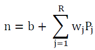
n: product of linear combination inputs.
b: absolute (fixed) bias.
wj : the weights associated with the inputs and they correspond to the parameters in the regression model.
Pj: input variables.
f(•) : the activation function used.
There are other formulas to describe artificial network inputs, including:
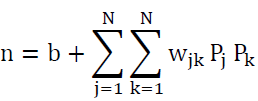
Higher Order (Second Order Form): It Is Described:
Delta rule (Π Delta (Σ): It is described by the formula:
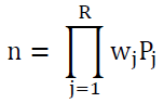
And the relationship represents the product of multiplying the weights with the input variables, and this formula is generally of little use in the fields of research (Bone &Asad, 2003).
Activation Function: It is also known as the transfer function because it converts the inputs through their interaction with the weights from one mathematical formula to another Figure 2. The activation functions include the following:
Log- Sigmoid Function: This function is considered the most widely used in the hidden layer nodes of neural networks. Its inputs are real values between (-∞,∞), while the function’s outputs for each node of the network are between (0,1) and the function formula is:
f(n)= (1+ e^(-n/T))-1
The derivative of the function is described by:
[f(n)] [1- f(n)]/ T =f.(n)
Where ((T) is a default parameter (Temp parameter)
The shape of the function when (T=1) is as follows:
Linear Function: This function is often used at the output layer and its form is: a= f(n)= n; Since the inputs are real values, the result of the function does not change, and its derivative is f.(n) = 1, and the graphical form of this function is as follows:
Hard Limit Transfer Function: The formula for this function is described as follows: a= f(n)
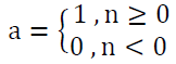
As the output of this function depends on the input, which is represented by the linear combination. If the input is greater or equal to zero, then the output of the function is equal to (1), otherwise the output of the function is equal to zero, and it is characterized by the absence of the derivative. This function is used in the case of classification models and the form of the function is Figure 4.

Figure 4 Linear Function
Threshold (Heaviside) function: The function is described as a= f (n)
It represents (n) the linear combination of the inputs, while the output of the function is equal to (1) when the linear combination is greater or equal to zero and when it is less than zero, the output is equal to (-1) and there is no derivative for this function and the form of the function is graphic Figure 5.

Figure 5 Threshold (Heaviside) Function
This function is also known as the symmetrical hard limit function.
Hyperbolic Tangent Function: The formula for the function is as follows
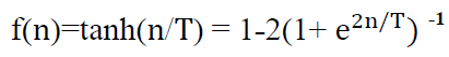
The inputs of this function are real values between (-∞,∞), while the outputs are between (-1,1) and the derivative of the function, which is used in estimating the parameters, is:
=[1- (f(n))2 ]/T f.(n)
or the derivative can be:
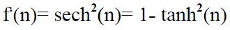
The function form is Figure 6.

Figure 6 Hyperbolic Tangent Function
Stages of Forecasting through Artificial Neural Networks
The process of Forecasting through artificial neural networks covers the following steps:
• Variables Selection: Success in designing neural networks depends on a clear understanding of the problem and knowing and selecting the input variables, as the problem is well represented, increasing the ability of neural networks to detect non-linear relationships between a number of different variables.
• Data Collection: Data is collected based on the problem studied and in a manner that suits the requirements of training the neural network, and that this information is from reliable sources.
• Data Preparation for Forecasting: This stage includes preparing the data for use in analysis and forecasting, as described in the paragraph above, as well as determining how to segment the time series into.
• Training Set: It is a set of time series data used to train the network to make Forecasting s, as this set is used to estimate weights. The number of models in the learning set, as described by Haykin (1994), which requires classifying observations with an acceptable error (ϵ), is described as N = ϵ/w, so (w) It represents the number of weights in the network, and the percentage that is chosen in the learning set must be of a certain size to give specifications and features to the variables for training the network so that the Forecasting is reliable.
• Test Set: It is part of the time series data and a sample that was not used in training. It tests the network’s predictability after the learning process. There is no scientific basis for determining the division of the data into two groups, learning and testing. 90% of the series data may be taken for learning and 10% for testing, or 50% may be for learning and 50% for the exam and some software sets 70% for learning and 30% for the exam (Wei, 1990).
• Validation Set: It performs a final monitoring to evaluate the training performance of the neural network in general, and choosing the number of data for this group must be appropriate to evaluate both training and testing in order to reach the best Forecasting (Tkacz, 2001).
• Network Architecture Determination: This part represents the basis for building the structure of the neural network, as it requires the network designer to have high skill and experimental experience in determining the factors by choosing the type of network, and to determine the architecture, the following steps are followed:
• Determination of Input Nodes: The selection depends on the number of explanatory variables that are described in the learning set, and the number of variables in the time series model depends on the formula described in terms of the shifted variables, meaning that  With a single Forecasting step, which is more preferable when building neural network Forecasting models.
• Selection of Number of Hidden Layer: In most applications of neural network prediction models, there is one hidden layer, and it is preferable to use it, and the sufficiency of one layer has been proven by Kolmogorov's superposition theorem, and practically, and from experimental studies to the present time, it indicates that networks with more than four layers (2) hidden) will not lead to improving results. Rather, it increases the time required and the probability of inefficiency of the estimated model, which leads to inaccurate prediction and its results cannot be relied upon (Anderson, 1995).
• Selection of Hidden Neurons: There is no direct formula that determines the number of nodes in the hidden layer, but there are some rules for determining it. The number of nodes for one hidden layer is determined equal to 75% of the number of cells of the input variables, or by specifying between (0.5) and (3) times the number of cells of the input variables. Or by using a rule called (geometric pyramid rule), which indicates:
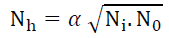
Nh: The number of nodes in the hidden layer.
Ni: The number of network inputs.
N0: The number of output nodes.
α: Multiplication factor: Its value depends on the degree of complexity of the problem to be solved and ranges between (0.5 < α <2).
There is another method proposed by Baum and Haussler (1989) where the number of nodes in the hidden layer is determined by the relationship:
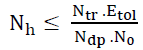
Ntr: The number of training samples (estimate).
Etol: Acceptable error.
Ndp: Number of input variables.
No: The number of output nodes.
There is also a formula for choosing the number of nodes in the hidden layer, which is represented by the Akike criterion (AIC) according to:
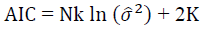
N: Number of estimation data.
k: The number of output nodes.
K: The number of parameters (weights) in the model.
The model that has the lowest value of the Akike criterion is preferred.
There is another criterion for determining the number of nodes in the hidden layer, known as Network Information Criterion (NIC), which takes the form:
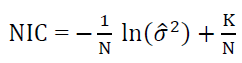
In general, the choice of the number of nodes in the hidden layer depends mainly on the number of input and output nodes (Hidayat & Wutsqa, 2020).
• Determination of Output Nodes: The presence of one output node is sufficient in the case of predicting one step in the neural network, but in the case of prediction for several steps, the number of nodes is corresponding and parallel to the subsequent prediction steps. Experiments have also shown that using one node gives good results compared to using more than one output node (Kneale et al., 2001).
• Selection of Activation Functions of Neurons: There are several formulas for activation functions that are related to the type of problem for which the model is being built and have been identified previously (Wei, 1990).
• Neural Network Training: The process of training neural networks for prediction is done by adjusting the network weights to obtain the lowest error, based on the back propagation (BP) algorithm and its modifications. The most important steps of training the network are:
• Select the Weight Initialization: It is considered the starting point for the training process, and small random values are often chosen for the weights and the absolute limit, which falls between (-1, 1). However, these values may not be good for the training process, so the initial value is calculated and taken for all network weights according to the formula: 1/√N where (N Number of network entries).
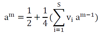
It is possible to calculate the initial weights between the hidden layer and the output layer through the multiple linear regression model. The model for the output node is in the formula:
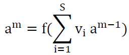
Vi: The weights are between the hidden layer and the output layer.
Assuming that the activation function is the logistic function, and through the use of the Taylor series for the function that is defined:
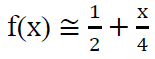
The linear relationship between outputs (am) and weights (Vi) is described as:
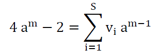
It represents a multiple linear regression model, as its features (weights) are estimated by the main regression methods (Kumar et al., 2008).
• Learning Rate and Momentum: The learning rate is one of the important factors in determining the size of the step needed to adjust the weights, while the momentum factor helps in balancing the training process, and this has been explained previously (Zhou et al., 2002).
• Stopping Criterion: It is a criterion that determines the end of the training process of the neural network through the error value E as well as the estimation error E_tr and the test and evaluation error E_(v ),E_t respectively. It may be determined by (5%) and according to what is intended to be processed in the network, this leads to reducing the error of the evaluation group, i.e. reaching an allowable error, and thus the training process ends (Makridakis et al., 1998).
• Implementation: The last step is one of the most important steps, as it tests the network in terms of its ability to adapt to changing conditions in the cycle, and the possibility of retraining and reaching the least square error when the data changes. It depends on the program used and equipped with means to train the neural network.
• The Applied Part: The neural network methodology is one of the modern methods that has high efficiency in giving good and satisfactory results.
Table 1 shows the number of inputs, the number of hidden nodes, the dimensions of the weights matrix (inputs - hidden), and the dimensions of the matrix (hidden - outputs) for all methods used.
| Table 1 Shows the Number of Inputs, the Number of Hidden Nodes, and the Dimensions of the Weight Matrix | ||||
| The model | Number of nodes | Number of hidden nodes | Input-Hidden Weight W1 | Hidden-Output Weight W2 |
| 9*2 | 3 | 9 | 9*3 | 9*2 |
| 9*2 | 3 | 9 | 9*3 | 9*2 |
| 9*2 | 6 | 9 | 9*3 | 9*2 |
Modeling according to the Box-Jenkins method:
The Box-Jenkins method (ARIMA) is one of the commonly used methods with high efficiency in modeling time series, which reflects the behavior of the time series, whether seasonal or non-seasonal Table 2.
| Table 2 Shows the Models for Temperatures | ||||
| The model | N | m | AIC | The model |
| (1,0,1) (0,1,1)12 | 60 | 2 | 77.35 | 55.65 |
| (0,1,1) (0,1,1)12 | 60 | 3 | 79.54 | 60.37 |
| (0,0,1) (0,1,1)12 | 60 | 2 | 78.84 | 63.15 |
| (1,1,1) (0,1,0)12 | 60 | 3 | 69.65 | 54.47 |
Temperature data for Basra Governorate was modeled for sixty months, then the best model was chosen based on the AIC standard Table 3.
| Table 3 Shows the Forecasting Values of the Average Temperatures along with the Forecast Periods According to the BJ Methodology | |||||
| Month | Predictive Value | forecast periods a = 0.05 | forecast periodsa = 0.01 | ||
| lowest | upper | lowest | upper | ||
| 1 | 13.3 | 12.4 | 15.4 | 12.4 | 14.2 |
| 2 | 10.5 | 9.4 | 22.2 | 9.4 | 11.6 |
| 3 | 16.4 | 13.9 | 20.3 | 13.9 | 18.9 |
| 4 | 28.1 | 24.3 | 31 | 24.3 | 31.9 |
| 5 | 32.8 | 31.2 | 35.3 | 31.2 | 34.4 |
| 6 | 39.9 | 35.5 | 43.6 | 35.5 | 44.3 |
| 7 | 47.2 | 44.7 | 50.8 | 44.7 | 49.4 |
| 8 | 46.5 | 44.6 | 49.3 | 44.6 | 48.4 |
| 9 | 42.2 | 37.8 | 45 | 37.8 | 46.6 |
| 10 | 31.6 | 30.5 | 35.3 | 30.5 | 32.7 |
| 11 | 21.2 | 20.5 | 22.7 | 20.5 | 21.9 |
| 12 | 19 | 15.4 | 21.4 | 15.4 | 22.6 |

where m represents the number of parameters estimated in the model.
Conclusion
1. Applying the neural networks method in various applied statistical studies due to the accuracy and flexibility that distinguish this method.
2. Expanding the study of the methodology of artificial neural networks because of its immunity, as it can address nonlinearity in data automatically and without the need for a previously proposed model.
3. The ability of the neural network to deal with large numbers of features with a different number and size of input variables, in addition to dealing with linear and non-linear relationships in the training process and for several times.
4. The artificial neural network (ANN) method is superior to traditional methods, as this superiority appears through the metrics used, and that the neural network methodology has the potential to process various types of linear and nonlinear data, as the artificial neural network method is easier and faster to use than traditional methods, and the neural network model Artificial back propagation of error gives a better representation of the data.
5. The neural network method is considered efficient and accurate, because it has the least sum of squared errors and low values of statistical metrics for most of the time series models used in this research. Analysis by this method requires less time and effort than classical forecasting methods, which assume difficult conditions for time series analysis.
6. To obtain more accurate results using artificial neural networks, attention must be paid to choosing a suitable architecture for the network represented by the number of input variables, hidden layer nodes, and activation functions used to process data in these nodes, and to determine the training that gives the least value for error.
References
Abdi, H., Valentin, D., & Edelman, B. (1999). Neural networks. 124, Sage.
Agami, N., Atiya, A., Saleh, M., & El-Shishiny, H. (2009). A neural network based dynamic forecasting model for trend impact analysis. Technological Forecasting and Social Change, 76(7), 952-962.
Indexed at, Google Scholar, Cross Ref
Al-Juboori, F.S., & Alexeyeva, N.P. (2020). Application and comparison of different classification methods based on symptom analysis with traditional classification technique for breast cancer diagnosis. Periodicals of Engineering and Natural Sciences, 8(4), 2146-2159.
Indexed at, Google Scholar, Cross Ref
Allende, H., Moraga, C., & Salas, R. (2002). Artificial neural networks in time series forecasting: A comparative analysis. Kybernetika, 38(6), 685-707.
Anderson, J.A. (1995). An introduction to neural networks. MIT press.
Indexed at, Google Scholar, Cross Ref
Atiya, A.F., El-Shoura, S.M., Shaheen, S.I., & El-Sherif, M.S. (1999). A comparison between neural-network forecasting techniques-case study: river flow forecasting. IEEE Transactions on neural networks, 10(2), 402-409.
Indexed at, Google Scholar, Cross Ref
Bone, R., & Asad, M. (2003). Boosting recurrent neural networks for time series prediction"m RAFI publication, International conference in Roanne, France,18-22.
Haykin, S. (1994). Neural networks, a comprehensive foundation. Macmillan College Publishing Company.
Hidayat, L., & Wutsqa, D.U. (2020). Forecasting the farmers’ terms of trade in Yogyakarta using transfer function model. In Journal of Physics: Conference Series, 1581(1), 012017.
Indexed at, Google Scholar, Cross Ref
Kneale, P., See, L., & Smith, A. (2001). Towards defining evaluation measures for neural network forecasting models. In Proceedings of the Sixth International Conference on GeoComputation, University of Queensland, Australia, available at http://www. geocomputation. org.
Kumar, P.R., Murthy, M.V., Eashwar, D., & Venkatdas, M. (2008). Time series modeling using artificial neural networks. Journal of Theoretical & Applied Information Technology, 4(12).
Makridakis, S., Wheelwright, S. C., & Hyndman, R. J. (1998). Forecasting methods and applications, John Wiley& Sons. Inc, New York.
Tkacz, G. (2001). Neural network forecasting of canadian gdp growth. International Journal of Forecasting, 17(1), 57-69.
Wei, W.S. (1990). Time series analysis. Univariate and multivariate methods. Addison. Wesley publishingcomp.
Zhou, Z.H., Wu, J., & Tang, W. (2002). Ensembling neural networks: many could be better than all. Artificial intelligence, 137(1-2), 239-263.
Indexed at, Google Scholar, Cross Ref
Received: 12-Sep-2023, Manuscript No. JMIDS-23-14002; Editor assigned: 14-Sep-2023, Pre QC No.JMIDS-23-14002(PQ); Reviewed: 22-Sep-2023, QC No. JMIDS-23-14002; Published: 26-Sep-2023