Introduction

The COVID-19 outbreak in early 2020 and its subsequent spread across the globe, forced countries to adopt policies to mitigate its impact. These policies included imposing lockdowns and travel bans. The crisis posed lots of uncertainties for investors and policymakers. Governments across the globe announced various stimulus packages to avoid the health calamity turning into an economic crisis.

In India, COVID-19 cases started emerging during the beginning of March 2020. Resultantly, the Government of India imposed one of the strictest lockdown on 23^rd March, 2020. This was an unprecedented crisis and the economic impact was felt across all markets. The investors and portfolio managers had to relook their strategies and realign asset allocations.

Various researches have established that asset risks and returns respond to major events. There have been studies to capture the impact of major events such as disasters (Kowalewski & Śpiewanowski, 2020), political events (Bash & Alsaifi, 2019; Shanaev et al., 2019) environmental conditions (Alawadhi et al., 2020; Guo et al., 2020); news (Li, 2018). The returns of different asset classes also responded to pandemic diseases such as Severe Acute Respiratory Syndrome (SARS) outbreak (Chen et al., 2007, 2009); Ebola Virus Disease (EVD); outbreak (Ichev & Marinč, 2018).

The high degree of uncertainty had an effect on the return and volatility of different asset markets, which include the stock market (Chaudhary et al., 2020), exchange rates (Iyke, 2020) and trade and economic growth (Vidya & Prabheesh, 2020). The oil market also experienced high turbulence due to the rise in uncertainty (Devpura & Narayan, 2020; Narayan et al., 2020). A sharp reduction in oil consumption because of lockdowns led to a drastic decline in crude oil prices in the international market, from USD 61 on 2nd January, 2020, to USD 12 on 28th April, 2020. Apparently, oil price movements play a key role in the performance of foreign exchange and stock markets of oil-importing economies, as shown by Prabheesh, et al., (2020). This uncertainty forced people to hold their liquid assets. Resultantly, money supply in the market was impacted, which further influenced the money and debt market. COVID-19 induced uncertainty in India; it distorted the dynamic interlinkages between different assets and markets, which included stock market, gold prices, exchange rates, oil prices, debt and money market returns. Thus, the present paper investigates whether and how these dynamic relations have evolved in the face of different waves of the COVID-19 pandemic in India.

In this study, the impact of different waves of COVID-19 crisis has been evaluated on different asset classes, by examining the return and volatility of return of these assets. The study has been undertaken on seven different asset classes, representing various assets for investments, which include Stock market, Gold, Currency, Oil, Cryptocurrency, Debt and Money market.

The current study is important for investor and portfolio managers, since it sheds light on information about the volatility structure of different asset classes, which in turn, will help in redesigning and rebalancing the portfolio under different market conditions.

Review of Literature

The theoretical link between different asset classes has been explored in earlier studies. For instance, the oil price–exchange rate nexus, states that a rise in oil price leads to depreciation of the currencies of importing economies, and shifts the wealth from oil-importing to oil-exporting countries (Salisu et al., 2020). Similarly, the nexus between oil prices and stock prices shows that a rise in oil price increases the cost of production and decreases economic growth, thereby leading to a decline in stock prices due to lower future earnings and dividends (Narayan & Sharma, 2011).

The literature on uncertainty and market movements shows that an increase in macroeconomic and policy uncertainty negatively affects economic growth, which in turn, reduces the demand for oil, as well as its price. Similarly, uncertainty is the key factor driving volatility in stock prices and exchange rates. In India, gold is used as jewelry, as reserve, and is also considered a precious metal (Yıldırım et al., 2020). There was a negative relationship between yen-dollar exchange pricing and gold prices. Levin, et al., (2006) examined whether or not gold is a long-term hedge against inflation in India, Indonesia, China, Saudi Arabia, and Turkey.

There has been growth in COVID-19 literature and its impact on different markets across the globe (Chaudhary et al., 2020; Gupta et al., 2021). The impact of COVID-19 uncertainty has adversely affected oil prices and returns (Devpura & Narayan, 2020), exchange rates (Rai & Garg, 2021), and stock returns (Haroon & Rizvi, 2020; Prabheesh et al., 2020; Rai & Garg, 2021). Studies have also been conducted on the performance of different sectors in India during COVID-19, from a business and economical perspective (Chaudhary et al., 2020). However, the current study tries to identify interrelations of different asset classes of varied nature. Besides this, the study also captures the behavior of markets during the first and second COVID-19 waves in India. The first COVID-19 wave started when cases started rising from March 2020, and peaked in September, 2020. The second COVID-19 wave commenced in April - May 2021 because of the surge of the delta variant, which was highly infectious and accompanied by high fatalities.

The present study addresses this issue in the Indian context. The reason for choosing India, for this research, is as follows; a) India has been severely impacted by the COVID-19 crisis, since there have been two major waves of COVID-19, and b) India is the sixth largest economy in the world and second largest in terms of population. Thus, our study contributes to the literature in the following ways; firstly, in understanding the behaviors of different asset classes under uncertainty; secondly, the response of different asset classes in both the waves and thirdly; in understanding the relationship of different assets under different economic conditions.

The remainder of the paper is organized as follows; Section 3 presents the data and methodology, Section 4 presents the empirical findings, while Section 5 discusses the empirical findings. Finally, the discussion and conclusion are presented under Section 6.

Data and Methodology

In this study, the daily data of Nifty, Gold prices, Three Month Treasury Bill Yield, Ten Year Government Security Bond Yield, Exchange Rate of Rupee-US Dollar, Bitcoin and Crude Oil Index are taken into account to represent respective asset classes (table 1).

Table 1 Asset Classes
Asset	Representation	Source	Symbol
Equity	It is represented by Stock market Index-Nifty. It is the index representing top 50 companies, across different sectors in National Stock Exchange of India	National Stock Exchange	LNIFTY
Gold	Prices of Gold per 10 gm	Multi Commodity Exchange India	LGOLD
Money Market	The yield of 3 Month T-bill represents the money market	Reserve Bank of India	L3MTBILL
Debt	The yield of 10 Year Government Bond represent Indian Debt market	Reserve Bank of India	L10YRGSEC
Currency	The Rs. /USD rate represents the currency market	Reserve Bank of India	LUSD
Cryptocurrency	The daily Bitcoin prices in rupees represent the crypto currency market	Investing.in	LBITCOIN
Oil	MCX COMDEX Crude Oil Index represents the Oil market and index is based on oil prices in MCX	Multi Commodity Exchange, India	LMCXOIL

The time period for this study comprises of 585 days, dating from 1st January, 2019 to 20th May, 2021. The time period has been divided into different phases in order to identify the volatility behaviour during these phases. They are as follows;

Phase 1: 1^st January, 2019 to 28^th February, 2020

This period has been considered as the pre-COVID-19 stage in India as in this stage, there were just three COVID-19 cases (Source: COVID-19india.org). It was from March 2019 that cases in India begun rising. Moreover, the year 2019 had been typical with no significant shocks in the economy.

Phase 2: 1^st March, 2020 to 16^th September, 2020

This has been considered as the first COVID-19 wave in India, which additionally saw the burden of one of the strictest lockdown across the globe. On 24^th September 2019, the active number of cases crested with nearly 100,000 cases coming in on a single day, and the quantity of active cases crossed 1 million.

Phase 3: 17^th September, 2020 to 28^th February, 2021

This phase saw a decline in COVID-19 cases and in this stage, unlocking of economic and business activities started across the nation. During this phase, the number of daily cases came down to 10,000 and active cases came below 150,000 in the country.

Phase 4: 1^st March, 2021 to 20^th May, 2021

During this phase, there was a second flood of COVID-19 in India, which was more infectious and more deadly than the first wave. The daily number of cases contacting COVID-19 was more than 400,000 and active cases crossed over 3.5 million. The pace of increase in the number of cases was additionally a lot quicker than the first wave, which prompted lockdowns once again in different parts of the country.

To capture the effect of different phases, a dummy variable was created to represent these phases and also, to identify the difference in volatility and return in these phases. The three phases during COVID-19 are denoted by dummy variables; d1, d2 and d3, whereas the pre-COVID-19 phase is assigned the value zero. as shows in Figure 1.

Estimation Techniques

The analysis of the performance of different assets during both COVID-19 waves in India is done through different statistical techniques such as descriptive statistics, GARCH (1,1), EGARCH(1,1), TGARCH(1,1) and GARCH-M models.

Descriptive Statistics & Correlation Analysis

The mean and median are taken as measures of central tendency. Standard deviation, skewness and kurtosis are used as measures of variability. Skewness and kurtosis are also used to identify the nature of volatility in the returns of assets. The Jarque–Bera test was conducted to confirm the normality of data. To get better insight into the return data of assets, a time series plot has been drawn.

The natural log returns of all the assets have been calculated using the formula below;

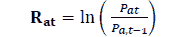
Rat=Daily return of assets a at day t; Pat=Closing price of asset at day t; P_a,t-1=Closing price of asset at day t-1.

A correlation analysis of daily market returns in different phases of the study was also conducted.

Unit Root Test

This test is used to check for the presence of stationarity in a time series data. The time series is said to be stationary if the distribution of time series is time invariant. This is a necessary condition for modelling the data for any analysis. The presence of stationarity in the time series data indicates that the mean, variance and covariance structure does not change over a period of time.

To check for stationarity, Augmented Dicky Fuller (ADF) test was applied (Dickey & Fuller 1981). The null hypothesis of ADF test is as follows;

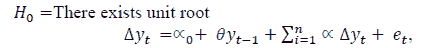
In the above equation, ‘y’ indicates the time series is time period t, αo is called the constant value, ‘n’ is the optimum number of lags and ‘e’ is known as the error term.

Granger Causality

Granger causality is a way to investigate causality between two variables in a time series. Causality is closely related to the idea of cause-and-effect, although it isn’t exactly the same. A variable X, is causal to variable Y, if X is the cause of Y or, Y is the cause of X.

The Granger Causality test has been used to test the relationship between various assets, and to establish a relationship that the return of one asset, can help in forecasting returns in another asset. For testing the granger causality relationship, the following equations have been used;

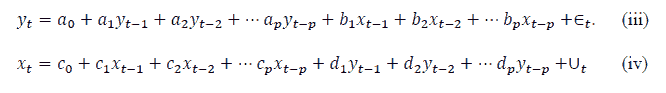
If, in the equation (iii) above all the coefficients of x, bi for i=1......l are significant then the null hypothesis, that x does not cause y, is rejected. Similarly in equation (iv) all the coefficients of y, di for i=1…l are significant, then the null hypothesis, that y does not cause x is rejected.

Based upon this, the relationship can be concluded, that is, whether or not any relationship exists at all. It can be Univariate if only in one equation in the hypothesis is rejected or bivariate, if in both the equations Null hypothesis is rejected or, No relationship if relationship is not rejected.

Estimating Mean Equation

To estimate the model, the mean return equation is first derived by fitting the ARIMA (p, q) model (Auto Regressive Moving Average Model). ARIMA (1, 1) has been taken as the best-fit model for fitting the conditional mean equation.

Conditional Mean Equation:

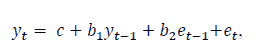
In the above equation, yt represents the conditional mean, c represents the intercept, represent the coefficient of AR (1), b₂ represents the coefficient of MA (1) and et represents the error at time t.

ARCH Effect Test

The ARCH-LM test (Auto Regressive Conditional Heteroscedasticity - Lagrange Multiplier Test) has been used to check for heteroscedasticity for residuals, and is used to check the presence of ARCH effect (Engle, 1982). To test for ARCH of order p, the following auxiliary regression model has been used;

In this, ‘u ’ is referred to as the square residual, which can be estimated by the mean regression model and ‘p’ represents the lag length in the residual regression model.

The null hypothesis of the ARCH-LM test is that there is no heteroscedasticity or, there is no ARCH effect;

GARCH Model

The Generalized ARCH (GARCH) model is a modification of the ARCH model. GARCH models are able to incorporate the effect of news and persistency. The models also are more parsimonious as compared to ARCH because of lesser parameters. The GARCH (p, q) model can be expressed as follows (Brooks, 2002);

Conditional Variance Equation (GARCH (1, 1)

In the equation (vii), are coefficients of the ARCH and GARCH terms, respectively, where ‘α’ (ARCH effect) estimates the response to shock or news in the market. ‘β’ (GARCH effect) measures the time it takes for any impact to die away, which can also be referred to as persistency. Greater α values depict higher sensitivity of volatility to new information, while greater β values depict greater amount of time for the change to die out (Rastogi, 2014). To have a stable model, a sum of (α+β) has to be less than one or else, the series will exhibit explosive behaviour; this is also an indication that series is not stationary.

Threshold GARCH (TGARCH) Model

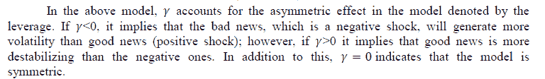
The standard GARCH model assumes there is symmetric behaviour of volatility on positive and negative errors, implying that both positive and negative news have the same impact on the volatility. However, it is believed that financial markets exhibit nonlinear behaviour to different news because of which there is a leverage effect, and this effect is not captured by a GARCH model. The reaction to different types of news can be incorporated into the GARCH model using a dummy variable. This feature introduced by Glosten, et al., (1993) was referred to as the TGARCH model and showed that asymmetric adjustment was an important consideration with asset prices. The form of the model is as follows;

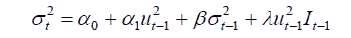
Where I is a dummy variable that takes the value of 1 when the news is negative, and 0 otherwise. The coefficient ?>0 and ? ? 0 shows the impact of leverage and also asymmetric shock in the equation depicted above.

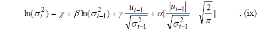
Exponential GARCH (EGARCH) Model

The alternative to the GARCH model is to use the EGARCH model, proposed by Nelson (1991). In this model, the non-negativity constraint does not need to be imposed and the asymmetries are also allowed for using the model below;

GARCH-in-Mean GARCH-M (Model)

In this class of models, the conditional variance enters into the conditional mean equation as well as the usual error variance part. The model identifies the effect of volatility on the return which is as follows;

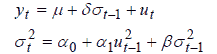
Here, yt is assumed to be the return of asset, and equation (x) suggests that the mean return is dependent on the past volatility. If parameter d is positive and significant, it means that the mean return increases when there is higher volatility in effect. d can also be attributed as a risk premium. However, if d is insignificant, it can be concluded that the return of an asset is not influenced by past volatility.

Empirical Results:

Descriptive and Correlation Analysis

The return of 585 days for the entire study period from 1^st January, 2019 to 20^th May, 2021 was plotted to identify the presence of volatility clustering in different markets. As observed from Figure 2, it can been seen that there was a high degree of volatility in returns during the months of March and April 2020, across all asset classes. The pattern of volatility clustering across different assets is also witnessed. To explore further, descriptive analysis was conducted in different phases. During the pre-COVID-19 phase, the daily average returns of all assets were positive, excluding the Money Market, where the daily average return of 3 Month T Bill was negative (-0.09%). During the same period, Bitcoin generated a daily average return of 0.29%, and it also had a high degree of daily volatility of 4.26%. During the pre-COVID-19 phase, it was observed that equity was negatively correlated with all assets except the 3 Month T Bill. Furthermore, oil prices during this phase witnessed high kurtosis indicating the presence of high leptokurtic distribution. During this phase, the Stock market (NIFTY) showed negative correlation with Gold, Rs/USD and G Sec.

In the first COVID-19 wave, the stock market, as expected, plummeted showing a negative daily average return (-0.03%), which was also accompanied by high volatility (2.51%). Besides the stock market, the money market was also the worst hit as the yield showed a sharp decline, with the daily average return (-0.28%) and volatility also rising (2.51 %). In addition to this, the oil market witnessed one of the highest volatility (86.42%) and kurtosis (69.95). This was primarily due to lockdowns imposed across the globe as a result of which the demand for oil plummeted. The daily return in the gold during this period rose to 0.13%. However, during the first COVID-19 wave, the stock market continued to show high negative correlation with Rs/USD exchange rate. One of the major reasons for Rupee falling to its 10 month low is attributed to FIIs (Foreign Institutional Investors) fishing out money from the Indian equity markets.

In phase 3, the Stock market and Oil Prices bounced back with the fall in active COVID-19 cases. However, the volatility and the fall in yield of 3 month T-Bill continued. Bitcoin also showed an upswing in returns (1.37%) with high volatility (4.92%). The gold return during this period showed a negative return (0.08%). As expected, gold once again showed negative correlation with the stock market. Once the stock market showed recovery, the rupee also showed signs of appreciation with FII coming back to markets. This phenomenon is also observed in the negative correlation of Rs/USD with Nifty (-0.46).

During the second COVID-19 wave in India, which was more lethal and infectious as compared to the first COVID-19 wave, all the asset classes in this study, other than currency, showed positive daily returns. During this phase, the lockdown was not a compulsion by the Central Government, but many prominent and bigger states like Maharashtra, Tamilnadu and Karnataka imposed strict lockdowns. The volatility observed during this period was lesser than the first COVID-19 wave. The behavior of markets was similar to the pre-COVID-19 phase, as the Stock market maintained its buoyancy, and the return of Stock market was negatively correlated with Gold, Rs/USD and GSec yields, which was similar to the pre-COVID-19 phase. This reflects the resilience of markets to COVID-19.

Table 2 Descriptive Statistics ( Jan1 2019 - Feb 28 2020)
	LNIFTY	LGOLD	L3MTBILL	L10YRGSEC	LUSD	LBITCOIN	LMCXOIL
Mean	9.19E-05	0.10%	-0.09%	0.04%	0.02%	0.29%	0.01%
Median	0.02%	0.09%	0.00%	0.05%	0.01%	0.03%	0.08%
Max	5.18%	3.60%	2.81%	0.98%	1.59%	20.08%	14.37%
Min	-3.78%	-2.36%	-3.18%	-1.21%	-1.02%	-15.60%	-6.40%
Std. Dev.	0.90%	0.83%	0.62%	0.29%	0.36%	4.26%	2.22%
Skew	0.58	0.32	-0.48	-0.26	0.41	0.36	0.58
Kurto	7.97	4.83	7.57	4.77	4.30	6.79	9.10
Obs	287	287	287	287	287	287	287
J-B Test	311.54	45.02	260.36	40.61	28.20	177.96	460.89
Prob	0	0	0	0	0	0	0

Table 3 Descriptive Statistics ( Mar 1, 2021 - Sep 17, 2021)
	LNIFTY	LGOLD	L3MTBILL	L10YRGSEC	LUSD	LBITCOIN	LMCXOIL
Mean	-0.03%	0.13%	-0.28%	0.03%	0.01%	0.15%	-0.07%
Median	0.15%	0.22%	0.00%	0.05%	0.05%	0.31%	0.32%
Max	8.40%	3.55%	12.19%	1.30%	1.41%	14.59%	718.84%
Min	-13.90%	-5.65%	-19.15%	-1.34%	-1.95%	-49.73%	-726.96%
Std. Dev.	2.51%	1.33%	2.74%	0.39%	0.45%	5.91%	86.42%
Skew	-1.44	-0.86	-3.12	-0.30	-0.54	-4.16	-0.1384
Kurt	10.83	5.47	29.15	5.64	5.66	37.86	69.95
Obs	142	142	142	142	142	142	142
JB Test	411.87	53.76	4275.28	43.47	48.72	7599.32	26527.85
Prob	0.00	0.00	0.00	0.00	0.00	0.00	0.00

Table 4 Descriptive Statistics ( Sep 18, 2021 - Feb 28, 2021)
	LNIFTY	LGOLD	L3MTBILL	L10YRGSEC	LUSD	LBITCOIN	LMCXOIL
Mean	0.28%	-0.08%	-0.06%	0.00%	0.00%	1.37%	0.45%
Median	0.34%	0.03%	0.00%	0.00%	0.00%	0.98%	0.67%
Max	4.63%	2.40%	6.94%	0.58%	1.61%	19.18%	8.15%
Min	-3.84%	-4.75%	-3.62%	-1.16%	-0.61%	-14.00%	-5.68%
Std. Dev.	1.13%	1.06%	1.16%	0.23%	0.29%	4.92%	2.07%
Skew	-0.43	-1.06	1.72	-0.91	1.63	0.08	-0.01
Kurt	6.10	6.62	14.88	8.44	10.81	4.91	4.29
Obs	107	107	107	107	107	107	107
J-B Test	46.30	78.86	683.07	146.97	319.42	16.51	7.31
Prob	0	0	0	0	0	0	0

Table 5 Descriptive Statistics ( Mar 1, 2021 - May 20, 2021)
	LNIFTY	LGOLD	L3MTBILL	L10YRGSEC	LUSD	LBITCOIN	LMCXOIL
Mean	0.02%	0.08%	0.14%	0.06%	-0.02%	0.15%	0.08%
Median	0.20%	0.06%	0.00%	0.07%	-0.06%	0.47%	0.13%
Max	2.30%	2.06%	2.73%	0.37%	1.17%	7.48%	4.93%
Min	-3.60%	-1.74%	-1.22%	-0.84%	-0.80%	-13.81%	-5.60%
Std. Dev.	1.19%	0.79%	0.66%	0.21%	0.41%	4.56%	2.40%
Skew	-0.50	0.25	1.26	-1.67	0.74	-0.64	-0.29
Kurt	3.21	3.04	6.56	8.43	4.08	3.70	3.31
Obs	49	49	49	49	49	49	49
JB-Test	2.17	0.53	38.97	83.08	6.90	4.31	0.88
Prob.	0.34	0.77	0.00	0.00	0.03	0.12	0.64

Table 6 Correlation Table Phase 1 : Pre Covid-19
	LNIFTY	LGOLD	L3MTBILL	L10YRGSEC	LUSD	LBITCOIN	LMCXOIL
LNIFTY	1.0000	-0.1487	0.0502	-0.0160	-0.3230	-0.1202	0.1006
LGOLD	-0.1487	1.0000	-0.1155	0.0538	0.4093	0.2118	0.0386
L3MTBILL	0.0502	-0.1155	1.0000	-0.1647	-0.0272	-0.0979	0.0903
L10YRGSEC	-0.0160	0.0538	-0.1647	1.0000	-0.0983	0.0157	-0.1976
LUSD	-0.3230	0.4093	-0.0272	-0.0983	1.0000	0.0739	0.1952
LBITCOIN	-0.1202	0.2118	-0.0979	0.0157	0.0739	1.0000	0.0332
LMCXOIL	0.1006	0.0386	0.0903	-0.1976	0.1951	0.0332	1.0000

Table 7 Correlation Table Phase 2 : First Covid-19 Wave (Increasing Cases)
	LNIFTY	LGOLD	L3MTBILL	L10YRGSEC	LUSD	LBITCOIN	LMCXOIL
LNIFTY	1.0000	0.0626	0.0199	-0.0075	-0.4608	0.2836	-0.0557
LGOLD	0.0626	1.0000	-0.0839	-0.0040	0.0844	0.2416	-0.0320
L3MTBILL	0.0199	-0.0839	1.0000	-0.2561	-0.1529	0.0389	0.0145
L10YRGSEC	-0.0075	-0.0040	-0.2561	1.0000	0.0368	-0.0303	0.0316
LUSD	-0.4608	0.0844	-0.1529	0.0368	1.0000	-0.2677	0.0533
LBITCOIN	0.2836	0.2416	0.0389	-0.0303	-0.2677	1.0000	0.0519
LMCXOIL	-0.0557	-0.0320	0.0145	0.0316	0.0533	0.0519	1.0000

Table 8 Correlation Table Phase 3: First Covid-19 Wave (Decreasing Cases)
	LNIFTY	LGOLD	L3MTBILL	L10YRGSEC	LUSD	LBITCOIN	LMCXOIL
LNIFTY	1.0000	-0.0478	0.1213	-0.0933	-0.3182	0.1035	0.2691
LGOLD	-0.0478	1.0000	0.0516	0.1768	-0.0638	0.1527	-0.2751
L3MTBILL	0.1213	0.0516	1.0000	-0.0560	0.1068	-0.0790	0.1322
L10YRGSEC	-0.0933	0.1768	-0.0560	1.0000	-0.1449	0.2611	-0.1852
LUSD	-0.3182	-0.0638	0.1068	-0.1449	1.0000	-0.1455	-0.0928
LBITCOIN	0.1035	0.1527	-0.0790	0.2611	-0.1455	1.0000	-0.0183
LMCXOIL	0.2691	-0.2751	0.1322	-0.1852	-0.0928	-0.0183	1.0000

Table 9 Correlation Table Phase 4 : Second Covid-19 Wave (Increasing Cases)
	LNIFTY	LGOLD	L3MTBILL	L10YRGSEC	LUSD	LBITCOIN	LMCXOIL
LNIFTY	1.0000	-0.0555	0.2515	-0.0046	-0.1236	0.3026	0.0746
LGOLD	-0.0555	1.0000	-0.0237	-0.0033	-0.0093	-0.0657	0.0211
L3MTBILL	0.2515	-0.0237	1.0000	0.3041	-0.0528	0.1543	0.0066
L10YRGSEC	-0.0046	-0.0033	0.3041	1.0000	0.2396	0.0237	-0.1998
LUSD	-0.1236	-0.0093	-0.0528	0.2396	1.0000	-0.0335	0.0735
LBITCOIN	0.3026	-0.0657	0.1543	0.0237	-0.0335	1.0000	-0.1348
LMCXOIL	0.0746	0.0211	0.0066	-0.1998	0.0735	-0.1348	1.0000

To model the volatility dynamics and causality of markets, various models were employed. Firstly, test for stationarity of data was conducted through ADF (Augmented Dicky Fuller Test), and the log return data of all asset classes was found to be stationary (Table 9) at level

Table 10 Unit Root ADF Test
	LNIFTY	LGOLD	L3MTBILL	L10YRGSEC	LUSD	LBITCOIN	LMCXOIL
T-Stats	-7.8423	-23.6406	-9.1589	-8.1935	-8.3473	-7.4385	-17.8444
P value	0.00	0.00	0.00	0.00	0.00	0.00	0.00

Granger Causality

Thereafter, the Granger causality test was applied to identify the causality pattern among different assets in different phases. As observed from the table, during the pre-COVID-19 phase 1, there existed a unidirectional influence of Nifty return on the return of Bitcoin and Rs-USD returns were granger causing Gold return. Whereas, the Rs/USD returns were influenced by G Sec returns. There was also an existence of unidirectional impact of G-Sec return on the return of Money market. In addition to this, a bidirectional causality between Oil and T Bill was observed. During Phase 2, a bidirectional causality between T Bill and Stock Market, and also between Bitcoin and G sec was observed. There was unidirectional causality as G-Sec and Rs/USD influencing Nifty and Bitcoin influencing Gold & Rs USD and Rs/USD influencing T Bills. Under phase 3, which was the recovery phase of COVID-19 in India, there was only unidirectional relationship of Gold on T bill, Rs/ USD on Gold. In Phase 4, during the second COVID-19 wave in India, there existed only bidirectional causality between GSec and Nifty. It is thus observed that the causality among different assets was highest during the first COVID-19 wave and subsequently, the causality in other phases among different assets was less.

Table 11 Granger Causality Among Asset Classes Across Different Phases
	D=0 Phase 1	D1=1 Phase 2	D2=1 Phase 3	D3=1 Phase 4
Null Hypothesis:	F-Statistic	F-Statistic	F-Statistic	F-Statistic
LGOLD does not Granger Cause LNIFTY	2.0618	2.0551	0.3319	2.3066
LNIFTY does not Granger Cause LGOLD	0.8143	0.8487	0.1251	0.6804
L3MTBILL does not Granger Cause LNIFTY	1.4187	4.4810**	0.0857	1.4707
LNIFTY does not Granger Cause L3MTBILL	0.1146	2.6809***	0.3433	0.7837
L10YRGSEC does not Granger Cause LNIFTY	0.6638	3.2106**	0.7805	3.1891**
LNIFTY does not Granger Cause L10YRGSEC	0.3019	2.1744	2.4757	6.6892*
LUSD does not Granger Cause LNIFTY	0.1396	4.0662**	0.0116	0.3295
LNIFTY does not Granger Cause LUSD	0.8158	1.5108	0.3402	0.6412
LBITCOIN does not Granger Cause LNIFTY	0.8045	1.5385	0.0713	0.4038
LNIFTY does not Granger Cause LBITCOIN	3.4834**	1.1178	0.7223	1.2503
L3MTBILL does not Granger Cause LGOLD	0.8295	1.5839	0.1787	0.4239
LGOLD does not Granger Cause L3MTBILL	0.3823	0.8141	3.8274**	0.0732
L10YRGSEC does not Granger Cause LGOLD	1.7460	1.9522	0.3366	0.3063
LGOLD does not Granger Cause L10YRGSEC	0.7160	0.2895	0.4871	1.7859
LUSD does not Granger Cause LGOLD	3.4213**	0.7973	5.1149*	0.8282
LGOLD does not Granger Cause LUSD	0.5191	0.7273	0.0659	1.6252
LBITCOIN does not Granger Cause LGOLD	2.0696	9.3087*	2.1997	0.5000
LGOLD does not Granger Cause LBITCOIN	0.6705	0.8228	0.1581	1.2912
L10YRGSEC does not Granger Cause L3MTBILL	3.2113**	0.9316	0.9389	0.5772
L3MTBILL does not Granger Cause L10YRGSEC	0.6688	0.5168	0.1825	0.7011
LUSD does not Granger Cause L3MTBILL	0.3698	3.6760**	0.8338	2.2378
L3MTBILL does not Granger Cause LUSD	0.8080	1.7940	0.1093	0.0057
LBITCOIN does not Granger Cause L3MTBILL	1.7284	0.6390	0.3224	2.4100
L3MTBILL does not Granger Cause LBITCOIN	0.7845	0.2973	0.9349	0.3338
LUSD does not Granger Cause L10YRGSEC	0.1166	1.4340	2.1238	0.5759
L10YRGSEC does not Granger Cause LUSD	2.5468***	1.0572	0.3518	1.6269
LBITCOIN does not Granger Cause L10YRGSEC	0.4861	6.2186*	0.5287	5.2717
L10YRGSEC does not Granger Cause LBITCOIN	0.7276	2.9063**	0.1543	2.3824
LBITCOIN does not Granger Cause LUSD	0.7674	2.8495**	0.2909	0.8975
LUSD does not Granger Cause LBITCOIN	0.3409	1.7943	0.2301	1.4778
LMCXOIL does not Granger Cause LNIFTY	1.8127	1.6233	0.5582	0.3211
LNIFTY does not Granger Cause LMCXOIL	0.7036	0.6486	1.6848	1.0680
LMCXOIL does not Granger Cause LGOLD	0.3029	0.9139	0.6217	3.7960**
LGOLD does not Granger Cause LMCXOIL	0.1140	4.6503*	1.1079	0.1195
LMCXOIL does not Granger Cause L3MTBILL	3.8789**	0.4792	0.6589	1.9049
L3MTBILL does not Granger Cause LMCXOIL	3.0349**	0.3134	2.3167***	0.4385
LMCXOIL does not Granger Cause L10YRGSEC	8.1393*	2.6688***	0.5235	0.0894
L10YRGSEC does not Granger Cause LMCXOIL	0.4752	0.7432	0.5613	0.0849
LMCXOIL does not Granger Cause LUSD	3.1461**	2.4385***	0.1269	1.9226
LUSD does not Granger Cause LMCXOIL	1.5626	0.2617	0.3066	1.4733
LMCXOIL does not Granger Cause LBITCOIN	0.2034	0.3745	0.6168	0.5266
LBITCOIN does not Granger Cause LMCXOIL	3.0651**	0.3490	0.5414	0.6940

Conditional Mean Equation

The ARIMA model was adopted (1, 1) which included a dummy for different phases as the conditional mean model. This is as follows;

In the above model  assumes a value of 1 and it represents Phase 2, which is a time period of the first COVID-19 wave from 1st March, 2020 to 16th September, 2020;  assumes a value of 1 and represents Phase 3, which is the recovery phase from COVID-19-1 and; d3assumes a value of 1 and represents Phase 4, which is the second wave of COVID-19 from 1st March, 2021 to 20th May, 2021. The pre-COVID-19 phase is represented by Phase 1 in which the value of d1, d2 and d3 is taken as zero.

The Null hypothesis was then tested to find out whether there is no ARCH effect in the residual of the mean equation by applying ARCH-LM test, and as observed from Table 11, all the asset markets showed the presence of heteroscedasticity across all series. This is also reflected in the graphs of asset returns which showed high clustering, and thus GARCH process is employed to model this heteroscedasticity.

Table 12 ARCH Effect
	LNIFTY	LGOLD	L3MTBILL	L10YRGSEC	LUSD	LBITCOIN	LMCXOIL
F-statistic	17.1190	4.2436	13.9435	8.9737	6.8250	2.6556	2.5134
P-Value	0	0	0	0	0	0.0711	0.0821

GARCH Model

The GARCH equation has been modified to capture the impact of volatility in different phases as follows;

In the equation above,  represents long-term unconditional variance, α represents ARCH effect β represents the GARCH effect, δ1, δ2 and δ3 represent the coefficient of a dummy variable for Phases 2, 3 and 4, respectively

Since the data was not normally distributed in many phases, the model was estimated by Student’s t distribution. The mean equation was obtained by fitting ARIMA (1, 1) model equation (xi) with dummy variables to capture the effect of different phases of COVID-19. By using the maximize log likelihood function, GARCH parameters were estimated, equation (xii) and dummy variables for different phases were introduced to find the effect of volatility in different phases.

It is observed from GARCH (1, 1) that all asset markets exhibited the ARCH effect, which was significant, thus indicating that volatility is influenced by past news. There was also the presence of GARCH effect across all asset classes, which indicates the persistency of volatility for the last day. Thus, the terms ARCH and GARCH explained the influence of volatility across all asset markets. It is also observed that the sum of ARCH and GARCH terms across all markets is less than 1. However, other than Bitcoin and Oil Prices, there was no significant change in volatility over different phases. A significant increase in Gold return in Phase 2, and a significant fall in Phase 3 is also observed. In addition to this, there was a significant increase in Stock market return, G Sec Market and Bitcoin in Phase 2, during the first COVID-19 wave. The Oil market showed change in volatility over all the three phases with volatility increasing substantially in Phase 2, and showed a significant decline in the other two phases, primarily because of demand coming back in economies across the globe.

Table 13 Garch Model
Variable	LNIFTY	LGOLD	L3MTBILL	L10YRGSEC	LRs/USD	LBITCOIN	LMCXOIL
C	0.0002	0.0010*	-0.0002	0.0004*	0.0000	0.0014	0.0018
D1	0.0018	0.0009**	0.0003	-0.0001	0.0000	0.0028	-0.0277
D2	0.0034*	-0.0024*	-0.0002	-0.0003**	-0.0002	0.0132**	0.0014
D3	0.0004	-0.0007	0.0007	0.0002	-0.0002	0.0007	-0.0022
AR(1)	-0.9749*	0.9688*	-0.4845*	0.9134*	0.8837*	-0.9673*	0.5583
MA(1)	0.9862*	-0.9954*	0.4295*	-0.9399*	-0.9308*	0.9798*	-0.6431
C	0.0000	0.0000***	0.0000	0.0000***	0.0000	0.0005*	0.1664*
ARCH(a)	0.0995*	0.1238**	0.2312***	0.1047**	0.0979*	0.2497*	0.3472*
GARCH(ß)	0.8423*	0.6720*	0.7217*	0.8649*	0.8621*	0.5462*	-0.0019
d1	0.0000	0.0000	0.0001	0.0000	0.0000	0.0001**	0.2826*
d2	0.0000	0.0000	0.0001	0.0000	0.0000	0.0003***	-0.1661*
d3	0.0000	0.0000	0.0000	0.0000	0.0000	0.0003	-0.1659*
a+ß	0.9419	0.7958	0.9529	0.9697	0.9600	0.7959	0.3452

The stability of the GARCH (1, 1) model was also observed by conducting ARCH LM test and it was found that no correlation exists in the residual (Table 13).

Table 14 ARCH LM Test
	LNIFTY	LGOLD	L3MTBILL	L10YRGSEC	LUSD	LBITCOIN	LMCXOIL
F-statistic	0.5602	0.4683	0.0479	0.1135	1.3968	1.1292	0.2297
P value	0.8466	0.9105	0.8267	0.7363	0.2236	0.2884	0.6319

T-GARCH Model

To capture the effect of asymmetric volatility in returns of different assets, T-GARCH (threshold GARCH) model has been applied. The model, also referred to as the Glosten, et al., (1993) model, has been modified to capture the effect of different phases by inserting a dummy variable coefficient for different phases as follows;

In the above equation,  represents the coefficient of past error term, which captures the impact of past news;  represents the coefficient of the dummy variable I, which will have a value of 1 if the past error term is negative, signifying the impact of negative news, and  represents the coefficient of GARCH term, signifying the persistency of the volatility, while δ1, δ2 and δ3 represent the coefficient of dummy variables for different phases.

The presence of asymmetric volatility in all assets, other than the oil market, was perceived. There is an increase in volatility with negative news in the Stock market, Money market and Bitcoin. However, in Gold, GSec & Rs/USD showed a fall in volatility because of negative news. This indicates that in negative environment Gold, G Sec & Currency are safer bets for investors seeking low risks.

Table 15 Tgarch Model
Variable	LNIFTY	LGOLD	L3MTBILL	L10YRGSEC	LUSD	LBITCOIN	LMCXOIL
	0.0000	0.0000	0.0000*	0.0000*	0.0000*	0.0006*	0.1775*
	-0.0169	0.1644*	0.1506*	0.1334*	0.1715*	0.0470**	0.2667
?	0.2153*	-0.1661*	0.3356*	-0.0807*	-0.1567*	0.4079*	0.3096
ß	0.7483*	0.8655*	0.5104*	0.8222*	0.8034*	0.4592*	-0.0007
d1	0.0000	0.0000	0.0000*	0.0000	0.0000	0.0001	0.2853*
d2	0.0000*	0.0000	0.0000*	0.0000	0.0000	0.0003**	-0.1774*
d3	0.0000	0.0000	0.0000	0.0000	0.0000	0.0002	-0.1772*

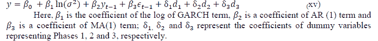
EGARCH Model

One of the advantages of deploying the EGARCH model in comparison to the GARCH model is that the log of conditional variance is always positive, irrespective of the values of the coefficient of equation. The model below is modified to incorporate the effect of different phases of COVID-19 as follows;

Here, represents the coefficient of GARCH term indicating the presence of persistency in volatility, depicts the leverage effect. If it is significant and negative, it implies the asymmetric effect of the news. Whereas if is non-significant, it implies that there is no difference in the type of news in the market and it exhibits symmetrical behaviour.

As observed from EGARCH (Table 15), coefficient for Nifty, T Bill, Bitcoin and Oil is negative indicating that bad news has a significant and larger impact than good news. However, in Gold, Rs/USD and G Sec, the coefficient is positive, indicating that with negative news coming in the market, volatility falls down.

Table 16 Egarch Model
Variable	LNIFTY	LGOLD	L3MTBILL	L10YRGSEC	LUSD	LBITCOIN	LMCXOIL
	-0.3423*	-0.5176*	-4.72837*	-1.3113*	-14.3584*	-2.0983*	-0.7363*
a	0.0052	0.1223*	0.1072*	0.1856*	0.3588*	0.4902*	0.6804*
	-0.2125*	0.1114*	-0.0478*	0.0530	0.0843**	-0.1666*	-0.2644*
	0.9644*	0.7149*	0.5435*	0.7494*	-0.2498	0.6184*	0.9584*
d1	0.0609*	0.0141	0.9856*	0.0364**	0.5944*	0.0466	0.3004*
	0.0142	0.0153	0.5977*	-0.0271	-0.7746*	0.1041**	-0.0711
	0.0147	0.0003	0.0423	-0.0670	0.3072	0.0616	-0.0030

GARCH-M Model

It is commonly understood in finance theories that with the increase in risk, the return in investments is also expected to increase. By applying the GARCH-M model, it was evaluated whether the increase in volatility leads to increase in return across different sectors. The modified equation used for identifying the impact of volatility in the return was;

It is observed that with the increase in volatility in Nifty, Rs/USD and Oil, there is a significant increase in return. However, in other asset classes, this behaviour of risk influencing the return is not observed.

Table 17 GARCH-M Model
Variable	LNIFTY	LGOLD	L3MTBILL	L10YRGSEC	LUSD	LBITCOIN	LMCXOIL
	0.0035*	-0.0011	0.0004	0.0003	0.0009*	-0.0048	0.3958**
	0.0342*	-0.0100	0.0029	0.0045*	0.0104	-0.0293	0.7738***
	-0.0024	0.0013	0.0015	-0.0003	-0.0001	0.0033	-0.3326
	0.0000	-0.0014	-0.0007	-0.0002	-0.0002	0.0151*	1.7678*
	-0.0043*	-0.0003	0.0016*	0.0001	-0.0006	0.0028	1.8239*
	0.1495	0.1162	-0.4466	0.8151*	0.9637*	-0.9671*	-0.2471
	-0.1646	-0.1004	0.3857	-0.8592*	-0.9968*	0.9806*	-0.0189

Discussion and Conclusion

This study focusses on the impact of COVID-19 waves on different asset classes in India. The study was divided into different phases in which Phase 1 was taken as the pre-COVID-19 phase from 1st January, 2019 to 28 ^th February, 2020. Phase 2, which is also referred to as a the first COVID-19 wave in India, from 1^st March, 2021 to 24^th September, 2021, witnessed high volatility across all assets, as depicted in descriptive analysis. The volatility across all asset classes is also accompanied with high kurtosis indicating the presence of extreme returns. It was observed that during the first COVID-19 wave in phase 2, the causality between different asset classes was much higher as compared to other phases. In phase 2, strict lockdown imposed across the nation gravely affected businesses and the economy.

This prompted the Government of India to announce stimulus packages to boost business. With cash flows suddenly drying up, corporates needed liquidity support, particularly in the short run. Resultantly, the Reserve Bank of India (RBI) resorted to the use of unconventional monetary policy tools in order to ensure adequate system level liquidity. Starting with the Long-Term Repo Operations (LTRO), RBI moved quite swiftly towards targeted liquidity provision, referred to as the Targeted Long-Term Repo Operations (TLTRO). The objective was to push money via banks at the current repo rate to sectors and entities experiencing liquidity constraints and/or hindrances to market access. The Government’s increased borrowing plan to overcome rising fiscal deficit even before COVID-19 struck, impacted the GSec yields. These changes brought about a significant impact in the Money market, Debt market Return and volatility. In phase 2, a very high degree of volatility was observed in Oil prices because of the fall in demand of oil across the globe. During this period, the Crude oil futures turned negative as there were more sellers than buyers in the market. Gold was the only asset class which provided positive returns with low volatility. This indicates the utility of Gold during crisis period.

It is also observed that all assets behave differently with the type of news coming in the market. While on one hand, negative news in the economy increases the volatility in Stock market, Oil Market and Bitcoin, on the other hand, in Gold and Currency, there is fall in volatility. Thus, Gold and Currency can act as assets for hedging. Both these assets also showed negative correlation with the Stock market and Oil market.

It is further observed that the Stock market, Currency and Oil market justifies taking more risk, if an investor is looking for higher return. This is in line with asset pricing theories such as CAPM (Capital Asset Pricing Model).

The study also reflects the resilience of asset return and volatility during the second COVID-19 wave. It is the Oil market which has significant impact and that too, a fall in volatility was observed in the oil market, which continued from the previous phase. This indicates that even though the second COVID-19 wave was more lethal and contagious, there was a reflection of positive sentiment. This can primarily be because of the launch of vaccines and it can also be attributed to the by-product of irrational exuberance (Schiller, 2015). Robert Schiller describes this conduct as the psychosomatic base of a speculative bubble. This speculative bubble is where information on value upsurges and converts into nonsensical investor energy. It spreads in the same manner as an infection. All the while, every individual enhances the story and justifies the price rise. Resultantly, the upsurge continued during the second and more lethal COVID-19 wave in India.

This study has important implications for portfolio and wealth managers in designing asset allocation for investors. It highlights the role of diversification in portfolio to reduce the impact of uncertainty in long term wealth creation. The study, over different phases of COVID-19, highlights the nature of different assets. It is noteworthy that none of the assets are insulated in all conditions. Therefore, Gold, as an investment, became a safe haven during crisis. However, this was not the case during the recovery phase. Even though the debt and money market are considered as safe investments, they can also be volatile during periods of uncertainty. Thus, portfolio diversification and rebalancing are the keys for sustainable and long term wealth creation.

References

Al-Awadhi, A.M., Alsaifi, K., Al-Awadhi, A., & Alhammadi, S. (2020). Death and contagious infectious diseases: Impact of the COVID-19 virus on stock market returns. Journal of behavioral and experimental finance, 27, 100326.

Crossref, GoogleScholar, Indexed at

Albulescu, C. (2020). Do COVID-19-19 and crude oil prices drive the US economic policy uncertainty?. 

GoogleScholar

Alfaro, L., Chari, A., Greenland A.N., & Schott, P.K. (n.d). Aggregate and firm-level stock returns during pandemics, in real time (Report No. w26950). National Bureau of Economic Research.

GoogleScholar

Asian Development Bank, Report No. 128, https://www.adb.org/publications/economic-impact-COVID-1919developing-asia

Bash, A., & Alsaifi, K. (2019). Fear from uncertainty: An event study of Khashoggi and stock market returns. Journal of Behavioral and Experimental Finance, 23, 54-58.

Crossref, GoogleScholar, Indexed at

Bollerslev, T. (1986). Generalized autoregressive conditional heteroscedasticity. Journal of Econometrics,31(3), 307-327.

Crossref, GoogleScholar, Indexed at

Bora, D., & Basistha, D. (2021). The outbreak of COVID-19?19 pandemic and its impact on stock market volatility: Evidence from a worst?affected economy. Journal of Public Affairs, e2623.

Crossref, GoogleScholar, Indexed at

Chaudhary, R., Bakhshi, P., & Gupta, H. (2020). The performance of the Indian stock market during COVID-19. Investment Management and Financial Innovations, 17(3), 133-147.

Crossref, GoogleScholar, Indexed at

Chaudhary, R., Bakhshi, P., & Gupta, H. (2020). Volatility in international stock markets: An empirical study during COVID-19. Journal of Risk and Financial Management, 13(9), 208.

Crossref, GoogleScholar, Indexed at

Chen, C.D., Chen, C.C., Tang, W.W., & Huang, B.Y. (2009). The positive and negative impacts of the SARS outbreak: A case of the Taiwan industries. The Journal of Developing Areas, 281-293.

Crossref, GoogleScholar, Indexed at

Chen, M.H., Jang, S.S., & Kim, W.G. (2007). The impact of the SARS outbreak.

Cochrane, J.H. (2008). The dog that did not bark: A defence of return predictability. The Review of Financial Studies,21(4), 1533-1575.

Devpura, N., & Narayan, P.K. (2020). Hourly oil price volatility: The role of COVID-19. Energy Research Letters, 1(2), 13683.

Dickey, D.A., & Fuller, W.A. (1979). Distribution of the estimators for autoregressive time series with a unit root. Journal of the American statistical association, 74(366a), 427-431.

Engle, R. (1995). ARCH: Selected readings. Oxford University Press.

Engle, R.F. (1982). Autoregressive conditional heteroscedasticity with estimates of the variance of United Kingdom inflation. Econometrica: Journal of the econometric society, 987-1007.

Estrada, R., & Arturo, M. (2020). Economic waves: The effect of the Wuhan COVID-19-19 on the world economy (2019-2020). Available at SSRN 3545758.

Fernandes, N. (2020). Economic effects of coronavirus outbreak (COVID-19-19) on the world economy. Available at SSRN 3557504.

Glosten, L.R., Jagannathan, R., & Runkle, D.E. (1993). On the relation between the expected value and the volatility of the nominal excess return on stocks. The Journal of Finance48(5), 1779-1801.

Crossref, GoogleScholar, Indexed at

Gourinchas, P.O. (2020). Flattening the pandemic and recession curves. Mitigating the COVID-19 Economic Crisis: Act Fast and Do Whatever, 31, 57-62.

GoogleScholar

Guo, M., Kuai, Y., & Liu, X. (2020). Stock market response to environmental policies.

Gupta, H., Chaudhary, R., & Gupta, S. (2021). COVID-19-19 impact on major stock markets. FIIB Business Review, 2319714521994514.

Haroon, O., & Rizvi, S.A.R. (2020). COVID-19: Media coverage and financial markets behavior?A sectoral inquiry. Journal of Behavioral and Experimental Finance, 27, 100343.

Crossref, GoogleScholar, Indexed at

He, Q., Liu, J., Wang, S., & Yu, J. (2020). The impact of COVID-19- 19 on stock markets. Economic and Political Studies, 8(3). Crossref, Google Scholar, Indexed at

Herwany, A., Febrian, E., Anwar, M., & Gunardi, A. (2021). The influence of the COVID-19-19 pandemic on stock market returns in Indonesia stock exchange. The Journal of Asian Finance, Economics and Business, 8(3), 39-47.

Crossref, GoogleScholar, Indexed at

Ichev, R., & Marin?, M. (2018). Stock prices and geographic proximity of information: Evidence from the Ebola outbreak. International Review of Financial Analysis, 56, 153-166.

Crossref, GoogleScholar, Indexed at

Iyke, B.N. (2020). COVID-19: The reaction of US oil and gas producers to the pandemic. Energy Research Letters, 1(2), 13912. Crossref, Google Scholar, Indexed at

Kowalewski, O., & ?piewanowski, P. (2020). Stock market response to potash mine disasters. Journal of Commodity Markets, 20, 100124.

Li, K., 2018. Reaction to news in the Chinese stock market: A study on Xiong?an Manag, 26(1), 200?212.

Mei, D., Liu, J., Ma, F., & Chen, W. (2017). Forecasting stock market volatility: Do realized skewness and kurtosis help? Physica A: Statistical Mechanics and Its Applications,481, 153-159.

Michelsen, C., Baldi, G., Dany-Knedlik, G., Engerer, H., Gebauer, S., & Rieth, M. (2020). Coronavirus causing major economic shock to the global economy. DIW Weekly Report,10(12), 180-182.

Narayan, P.K., & Sharma, S.S. (2011). New evidence on oil price and firm returns. Journal of Banking & Finance, 35(12), 3253-3262.

Crossref, GoogleScholar, Indexed at

Nelson, D.B. (1991). Conditional heteroskedasticity in asset returns: A new approach. Econometrica: Journal of the Econometric Society, 347-370.

Prabheesh, K.P., Padhan, R., & Garg, B. (2020). COVID-19 and the oil price?stock market nexus: Evidence from net oil-importing countries. Energy Research Letters, 1(2), 13745.

Rai, K., & Garg, B. (2021). Dynamic correlations and volatility spillovers between stock price and exchange rate in BRIICS economies: Evidence from the COVID-19 outbreak period. Applied Economics Letters, 1-8.

Rastogi, S. (2014). The financial crisis of 2008 and stock market volatility?analysis and impact on emerging economies pre and post crisis. Afro-Asian Journal of Finance and Accounting4(4), 443-459.

Crossref, GoogleScholar, Indexed at

Salisu, A., & Adediran, I. (2020). Uncertainty due to infectious diseases and energy market volatility. Energy Research Letters, 1(2), 14185.

Shanaev, S., Shuraeva, A., & Ghimire, B. (2020). The financial pandemic: COVID-19 and policy interventions on rational and irrational markets. Available at SSRN 3589557.

Shiller, R.J. (2015). Irrational exuberance. Princeton university press.

Tripathy, N. (2017). Do BRIC countries stock market volatility move together? An empirical analysis of using multivariate GARCH models. International Journal of Business and Emerging Markets,9(2), 104-123.

Crossref, GoogleScholar, Indexed at

Verma, R.K., Kumar, A., & Bansal, R. (2021). Impact of COVID-19-19 on different sectors of the economy using event study method: An Indian perspective. Journal of Asia-Pacific Business, 22(2), 109-120.

Crossref, GoogleScholar, Indexed at

Vidya, C.T., & Prabheesh, K.P. (2020). Implications of COVID-19 pandemic on the global trade networks. Emerging Markets Finance and Trade, 56(10), 2408-2421.

Crossref, GoogleScholar, Indexed at

Yildirim, H., Alola, A.A., & Sengelen, H.E. (2021). The causal nexus of interest rate policy and gold market: The case of Turkey. Journal of Public Affairs, 21(1), e2142.

Crossref, GoogleScholar

Zahedi, J., & Rounaghi, M.M. (2015). Application of artificial neural network models and principal component analysis method in predicting stock prices on Tehran Stock Exchange. Physica A: Statistical Mechanics and its Applications, 438, 178-187.

Crossref, GoogleScholar, Indexed at

Received: 18-Dec-2021, Manuscript No. AAFSJ-21-9845; Editor assigned: 20-Dec-2021, PreQC No. AAFSJ-21-9845 (PQ);Reviewed: 07-Jan-2022, QC No. AAFSJ-21-9845; Revised: 11-Jan-2022, Manuscript No. AAFSJ-21-9845 (R); Published: 18-Jan-2022