Keywords

Credit Risk, Diversification, Mergers and Acquisitions, Actuarial Model.

JEL Codes

G34, D81

Banking Crisis And Financial Deregulation In Japan

After World War II, banks in Japan had been heavily regulated by the Ministry of Finance. Interest rates, scope of business and foreign exchange were strictly regulated. As a result, competition was very limited and customers viewed banks indifferent from each other. Under the strict regulated system, banks are fully guaranteed by the Ministry of Finance. That is, banks can never fail under this system. The system proved it to be quite efficient in building Japan after World War II as evidence reveals that there were no major bank failures after the World War II up until around mid-1994.

Japan started deregulated its financial system in 1970s. The deregulation and liberalization were built around the motivation to make Japan a major world financial centre. However, transforming Japanese financial system in to the US-style system is not an easy process given existing cultures and tradition of Japanese financial system. One unique characteristic of Japanese financial system before deregulation in 1970s is the low level of consumer credit. Young workers had to save to build the house given such scarce consumer financing. Overall saving rate of Japanese population was thus higher than that of most developed countries. On the other hand, firms in the real sector were deeply in debt because the system encourages real sector corporations to heavily borrow with the main objective of injecting the economy with high level of investment.

The ratio of the financial liabilities of the real sectors to total Gross National Product (GNP) has been rapidly increasing after World War II through the financial deregulation period. Japanese banks were treated as an intermediary that channels surplus household saving to industrial sectors. Therefore, Japanese banks acted more like providers of public financial services than competitive private sector intermediaries. Given such uniqueness of Japanese financial system, the authority decided to move with the financial reform policy by using a stepwise basis. Since the enforcement of the Financial System Reform Law of 1992 in April 1993, banks and other depository institutions are allowed to compete with securities firms via subsidiaries.

The deposit insurance system was established in 1971 to act as a safety net for banking system in Japan. The deposit insurance law was later revised in 1986 and enacted in March 1987. It specified that the Deposit Insurance Corporation (DIC) can deal with failed banks under two options: Liquidation and financial assistance. The insurance amount under the liquidation option is up to ten million yen for each depositor. The loss amount above this upper limit might be recovered depending on the remaining value of the failed bank. Under the financial assistance option, the business of a failed bank would be transferred to an assuming bank. The DIC also transfers fund to an assuming bank as a financial assistance provision. Before the financial crisis, the insurance fund hold by the DIC was only 300 million yen, which was far too small compared to the actual deposit amount of banking system in Japan.

Japan began to experience major bank failures after mid-1994. In December 1994, two urban credit cooperatives; Tokyo Kyowa and Anzen, went bankrupt with a combined deposit of 210 billion yen. To avoid bank runs, the Ministry of Finance and the Bank of Japan decided to resolve the problem of these two failed banks by choosing financial assistance option, but there was no financial institution willing to be an assuming bank. As a consequence, the new bank named Tokyo Kyoudou Bank (TKB) was established to assume the assets and deposits of the two failed credit cooperatives.

In 1995, Daiwa Bank, an internationally active city bank was ordered by the US regulators to close all its operations in the US market. In that same year, seven Junsen companies or housing loan corporations, non-bank institutions providing heavy lending to real estate developers, also went bankrupt, with the estimated total loss of 6,410 billion yen. In 1997, two major banks; Nippon Credit Bank and Hokkaido Takushoku Bank, had become insolvent. The contagion effects continued to grow among financial institutions in Japan. In fact, during the month of November 1997, major financial institutions in western Japan became insolvent almost on a weekly basis. These failed financial institutions include Sanyo Securities, Hokkaido Takushoku Bank, Yamaichi Securities and Tokuyo City Bank.

In 1998, Long Term Credit Bank of Japan and Nippon Credit Bank, two of the three long-term credit banks, had become bankrupt in October and December, respectively. This is the largest bank failure in Japan. The banks were nationalized by the public funds with the total amount of 60 trillion yen, more than 12% of GDP. The Financial Reconstruction Committee (FRC) sold the nationalized Nippon Credit Bank to a consortium comprising three Japanese companies: Soft Bank, Orix and Tokyo Marine and Fire Insurance, in September 2000. The new bank was later named Aozora Bank. In March 2000, Long-Term Credit bank was sold to an international group led by US based Ripplewood Holdings. This is the first time in the history that a Japanese bank is owned by a foreign firm. With new management and services, Ripplewood Holdings renamed the bank to Shinsei Bank in June 2000. In February, 2004, the IPOs of Shinsei Bank is held. Shinsei Bank later exchanged its long-term credit banking license for a standard commercial banking license.

Incentives For Consolidations

After the financial crisis during 1990s, Japanese financial system has undergone a credit crunch period, during which time bank loans show negative growth rate until 2000. The Japanese financial system has also undergone a major structural change and consolidation. This is partly due to the consequences of deregulation and internationalization in the mid-1970s. Ever since, several bank mergers and acquisitions have taken place as a response to an increasing competition from abroad. The government also encouraged the mergers of weakened banks and the purchase of nationalized insolvent bank.

The financial reform was also necessary due to the collapse of the bubble economy, during which time most banks in Japan faced with increasing amount of bad debts and relatively poor profitability. The declining real estate prices during the financial crisis period contributed to huge amount of NPLs that almost all financial institutions experienced. Since the bursting of bubble economy in 1991, the land prices started to decline and continued to decline for 15 consecutive years¹. Moreover, liquidation of NPLs through securitization was not made possible until 1998. Even that so, the liquidation of NPLs worsened the losses to banks because NPLs must be sold at extremely discounted prices. Bad debt experiences have influenced banks to change their lending behaviors by taking into account risk assessment process more stringently when evaluating borrowers. Meanwhile, the regulators began to apply quantitative method to evaluate and monitor credit risk or expected default probability of each financial institution. The aggregated credit risk measure at the industry level can be used to reflect the overall stability of the financial system and assess the effectiveness of the government policy on financial system.

The return on assets at major Japanese banks averaged -0.1% during the year 1993 to 1998, compared to an average of 1.2% for the 22 largest US banks (Drake & Hall, 2000). To improve profitability, cost saving through economies of scale must be achieved. Merger and acquisition were viewed as a way to achieve economies of scale and improve profitability. Merger could also enhance the bank’s ability to write off non-performing loans. Up to 2004, ten leading banks have merged to create five mega banks, which include Mizuho Financial Group, UFJ Financial Group, Sumitomo Mitsui Financial Group, Tokyo-Mitsubishi Financial Group and Resona Holdings. On January 1, 2006, Tokyo-Mitsubishi and UFJ merged to form the Bank of Tokyu-Mitsubishi UFJ, the World’s largest bank, with a combined asset of approximately $1.7 trillion, left the Japanese banking industry with only three gigantic banks. The Bank of Tokyo-Mitsubishi UFJ has nearly 80,000 employees and 1000 branches around the world. Additional chronology of Japanese bank mergers and acquisitions is summarized.

Several articles applied Data Envelopment Analysis (DEA) framework to measure and report efficiency comparison in Japanese Banking before and after merging. Even though bank consolidation has been viewed as a key means of improving efficiency, an average efficiency score for a banking industry did not improve much from 1998 to 1999. Harada (2005) found that Tokai Bank’s efficiency score declined from 1 to 0.354 after merging with UFJ in 2001. This is due to the fact that UFJ had a very high level of bad debts, nearly 10% of the loans on its book. Therefore, a consolidation of an efficient bank with an inefficient bank does not create an efficient bank. Moreover, a merger of both inefficient banks would not lead to a more efficient bank either. An example of this result is a consolidation of Daiwa and Asahi.

Indeed, bigger does not always mean better in terms of efficiency. Nonetheless, mergers still take place as part of an effort to increase comparative advantage in banking system. Thus, incentives for bank consolidation in Japan might not be solely for efficiency improvement, but more toward combining unhealthy bank with the ones whose financial statements are in a better shape. In other words, Japanese banks decided to merge to seek for a more diversified loan portfolio, which could lower credit risk of their combined loan portfolio. The estimated bad loan is larger than $500 billion as a result of the collapse of Japan’s real estate market in the early 1990s and a cultural credit granting from Japanese bank to insolvent firms even when they made negative profits. To that extent, an effective credit risk management is required for the consolidated bank to be able to improve profitability.

Given the Basel Committee’s new Capital Accord on capital adequacy, the banks are subjected to an additional cost of bankruptcy reflecting the level of credit risk exposure. Consequently, to improve cost efficiency, the bank must improve the quality of its loan through enhancing credit underwriting technology and utilizing better credit information. Therefore, bank consolidation does not only mean balance sheet consolidation, but also refers to merging technology and information across banks.

Credit scoring has been considered one of the important tools for improving credit quality because it could reduce processing time for loan approval process and increase consistency and accuracy of loan approval decisions. Ono argues that credit scoring model is most useful for a relatively large bank because a larger bank can cost efficiently create and manage models as well as better diversify its loan portfolio. If this is the case, a larger bank through merger should benefit more from credit scoring model; and thus, should be able to achieve better quality of the loans on its book. Moreover, consolidation should also bring benefits of better diversification, including geographical diversification and economies of scale to consolidated bank under portfolio theory. As long as risks of consolidated banks are not perfectly correlated, a larger and more diversified loan portfolio should lead to lower probability of bankruptcy among consolidated banks and create a healthier banking system. However, some may argue that a larger bank due to consolidation may take on more risky activities because of too-big-to-fail behavior.

The results of empirical studies of bank diversification are interestingly mixed. Goetz, Laeven & Levine (2016) evaluate the impact of the geographic expansion of a Bank Holding Company (BHC) across US Metropolitan Statistical Areas (MSAs) on BHC risk. Their results suggest that geographic expansion materially reduces risk and that geographic diversification does not affect loan quality. The results are therefore support the arguments that geographic expansion lowers risk by reducing exposure to idiosyncratic local risks and prove against the arguments that expansion, on net, increases risk by reducing the ability of BHCs to monitor loans and manage risks. Gulamhussen, Pinheiro & Pozzolo (2014) study the relationship between bank internationalization and risk in the period leading to the financial crisis of 2007-2008. For a sample of 384 listed banks from 56 countries, they calculate two measures of risk for the period from 2001 to 2007-the Expected Default Frequency (EDF), a market-based and forward-looking indicator and the Z-score, a balance-sheet-based and backward-looking measure-and relate them to the degree of banks’ internationalization. They find robust evidence that international diversification increases bank risk. Doumpos, Gaganis & Pasiouras (2016) use an international sample of commercial banks and find that diversification in terms of income, earning assets and on-and off-balance sheet activities influences positively their financial strength. They also find that income diversification can be more beneficial for banks operating in less developed countries compared to banks in advanced and major advanced economies. In addition, they find that income and earning assets diversification can mitigate the adverse effect of the financial crisis on bank financial strength. Batten & Vo (2016) investigate risk shifting in commercial banks in Vietnam and find that commercial banks shifting to non-interest income activities face higher levels of risk. This finding is contradict to a common belief that diversification can result in risk reduction and improve stability.

However, these papers consider diversification from the context of international, geographic, income or asset diversification. To provide an alternative view of diversification from the context of credit risk, this paper proposes a theoretical model to prove that credit risk diversification is a consolidation incentive for Japanese banks. The main hypothesis to be tested is whether the merger and acquisitions have a positive impact on the credit risk of individual Japanese banks. In other words, whether a consolidated bank are less prone to insolvency given its larger portfolio diversification.

Credit Risk Measurement

Although the development of credit risk measurement is still far behind what have been developed for market risk, the economic capital requirement imposed by the Basel Committee on Supervision has made the credit risk measurement become notably important. Significant advanced tools for measuring credit risk have become available; for example, Credit Metrics by Morgan (Morgan, 1997), Credit Risk by Credit Suisse First Boston (CSFB, 1997), Credit Portfolio View by Wilson (1997a, 1997b, 1997c & 1997d); Mckinsey (1998) and KMV (Kealhofer, 1995). However, these tools lack of convergence on any one method.

Applying Value at Risk to a loan portfolio requires different assumptions from those used for measuring market risk of other trading portfolios. First, the risk associated with a bank loan portfolio should be measured by volatility of credit losses not volatility of credit returns because there is almost no potential upside gain on loans but a substantial downside loss. Second, since the credit loss distribution is not normal, likely to be positively skewed with fatter tails, the unexpected loss is not well approximated by some multiples of the portfolio’s standard deviation of losses. If the loan values are assumed to be normally distributed, the result of credit VaR tends to be underestimated. Third, while it is common to calculate market VaR by subtracting the portfolio’s expected loss from its maximum potential loss within a given confidence interval, this is not a common practice when calculating credit VaR because of zero expected loss assumption used in most standard market risk calculation. While zero expected loss is a justified assumption for market risk calculation where the holding period is rather short, it is not an appropriate assumption for credit risk calculation because the loan portfolio has almost no potential for upside gain but considerable downside loss. Thus, the expected loss is an essential component for credit VaR calculation. Fourth, we are interested in how market rate changes will impact the value of the trading portfolio when calculating market VaR whereas we are interested in how changes in credit quality will affect the value of the loan portfolio and the value of economic loss should credit events occur. Therefore, similar to market risk measurement where assumptions regarding the impact of market rate changes on the value of trading portfolio are crucial, credit risk measurement requires appropriate assumption regarding the impact of credit events on the value of loan portfolio. Specifically, when calculating credit VaR, we are interested in two random variables; frequency and severity of credit losses, which could be referred to as default probability and loss given defaults.

To model the joint credit loss distribution across all loans in the portfolio, estimation of correlation between credit events for different borrowers in the portfolio is needed. Under the assumption that credit events between borrowers are independent, credit risks can be diversified away for a large enough portfolio. This is not an appropriate assumption because such a well-diversified credit risk portfolio is not observed in practice no matter how large the loan portfolio is. Assuming that credit events between borrowers are constant across all borrower segments is not appropriate either because the default correlations between borrowers with different rating or between borrowers from different segments are less likely to be equal across portfolio. The idiosyncratic risk factors such as firm-specific or industry-specific risks are not correlated with each other; and thus, they do not contribute to the default correlations and can be diversified away whereas the risks associated with common factors are not diversifiable. However, correlations are expected to be higher between firms within the same industry than between firms from different industries. Therefore, diversification across industries can result in reduction in loss volatility. Such diversification impact is what we would like to model in this paper.

Multi-factor model can be used to determine default correlations of the loan portfolio. Since default events are highly related to underlying macro-economic cycle, macroeconomic variables such as GDP and unemployment rates can be used as explanatory variables in models predicting default rates. The correlations between segments are derived by assuming that average default rates by segment are driven by macro-economic factors. The choice of explanatory variables may differ depending on the types of loan portfolio, credit concentration of the loan portfolio or the country in which the financial institution is operating. For instance, Shimizu & Shiratsuka (2000) used real estate price index as one of the explanatory variables to estimate credit risk of Japanese Bank during the bubble period.

Alternatively, actuarial model used in property and liability insurance industry can be used to measure credit risk of a loan portfolio. Similar to insurance portfolio, a loan portfolio is consisted of a large number of individual risks, each with a low probability of loss occurrence.

Methodology

With its advantage of minimal data requirement, this paper develops an actuarial model to measure credit risk of a merged bank. Another advantage of using an actuarial model is that it is not subject to precision problems that can arise from simulation-based approach. The default rate is treated as a continuous variable. The continuous default loss distribution can be specified by obligor default rates and default rate volatilities. This is analogous to pricing stock option in which the data of both stock price and stock price volatility are required. An alternative to obtain default rates is to adopt default statistics published by rating agencies in a particular market or country. One-year default rate can significantly vary depending on macro-economic factor. For example, during economic recession period, the default rates for a given rating category tend to be higher than their average level.

To take into account the impact of common factors, we incorporate the default rate volatility into specifications of default rate rather than directly import default correlations derived from macro-economic model. This is considered a superior approach due to the lack of empirical data on default correlations, the difficulty in verifying the accuracy of macro-economic model and the instability of default correlations for a longer time horizon. The default rate volatility for a given rating category can be calculated as a standard deviation of historical default rates. Since the loan portfolio can have concentrations on particular industry sectors, the model used in this paper allows for such concentration risks to be captured using sector analysis. Each obligor in the portfolio can be assigned into a specific single sector representing a collection of obligors who are influenced by the same common factor. The concentration risk of the loan portfolio should be lower as the number of sectors increases. In other words, the degree of diversification increases with the number of sectors. Other required input data to generate the credit loss distribution are credit exposures and recovery rates. Given the credit loss distribution, we will be able to determine the size of credit loss for a given confidence level. Scenario analysis can later be applied to identify extreme loss.

In this paper, credit risk is defined as potential future credit loss due to credit events and credit VaR as the maximum possible loss for a given position of a portfolio given a certain confidence level over a specified time horizon. There are two distinct definitions of credit losses: Expected losses and unexpected losses. The expected loss is simply an expected value of loss calculated from a loss distribution and can be represented by the following formula:

Expected Loss= (Probability of Default) x (Exposure at Default) x (100%-recovery rate)

The portfolio expected loss can be calculated by summing expected losses of individual loans in a portfolio. The portfolio expected loss represents the amount of credit reserve that the bank should have on its book.

Actuarial methods are increasingly used and accepted by auditors and regulators as a means to determine a bank’s reserve. Similar to insurance business, expected loss is an important indicator determining the adequacy of product pricing model. The unexpected loss is referred to as the difference between maximum possible loss and expected loss. Indeed, credit VaR is the unexpected loss of the loan portfolio and represents the additional economic capital that the bank should hold against a given portfolio above the level of credit reserves because the actual credit losses in any given period could be significantly higher than the expected level.

Based on actuarial techniques, an aggregate loss distribution is generated from credit loss frequency and severity distributions. There are several possible choices for frequency distribution. When each obligor is assumed to have fixed default rate, each obligor either defaults or does not default. That is, the probability generating function of the number of defaults for each obligor follows the Bernoulli distribution; default occurs with the probability q and no default with the probability 1-q.

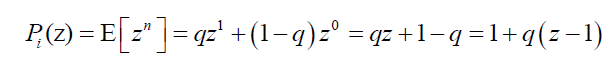
When there are N obligors in the portfolio, the probability generating function becomes:

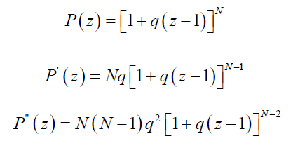
With the mean and variance of Binomial distribution as follow:

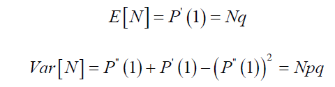
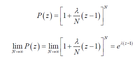
Therefore, the binomial distribution has the mean larger than the variance, which is not very pragmatic for loss event distribution. With some parameter transformation, we can obtain the probability generating function for Poisson distribution. For both distributions to have the same mean and maximum number of default events, the following parameter transformation is needed.

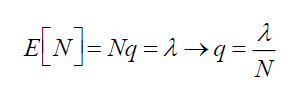
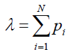
Where λ represents the expected number of default events in one year from the whole portfolio. That is,

Substitute q into the probability generating function of the Binomial distribution and taking N to the limit, we can obtain

This is the probability generating function of the Poisson distribution, which can be expanded with Taylor series to obtain the probability mass function of the Poisson distribution as follows:

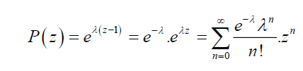
Thus,

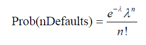
The Poisson distribution has a unique property that the mean and variance are both equal to λ. This is a drawback of the Poisson distribution when applying to a loan portfolio because historical data suggests that the variance of credit loss is larger than its mean. However, this result is obtained from the assumption of fixed default rates. The default rates can be allowed to be uncertain to reflect the fact that observed default probabilities are volatile over time. The volatilities in default probabilities could be correlated with the common factors such as the state of economy. Thus, allowing for such default uncertainty can incorporate into the credit risk model the impact of common factors on the default likelihood of obligors within a portfolio.

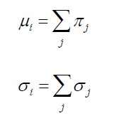
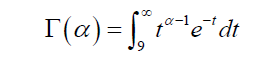
Sector analysis can be used to incorporate such default rate volatilities into the model by assigning a specific sector i to each obligor. Each sector is treated as a portfolio and independent from other sectors. Thus, the whole portfolio is consisted of several sub-portfolios as sectors. The obligors in the same sector are influenced by the same common factor. In each sector i, the expected number of default is treated as a random variable Assume that is Gamma distributed with parameters r_i and β_i, the mean and variance of are equal to:

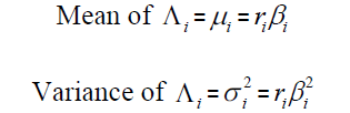
The parameter estimates for r_i and β_i are

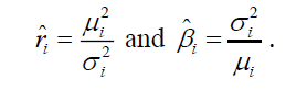
If each obligor j in sector i is assumed to have the probability and volatility of default equal to π _j and σ _j respectively; where both π_j and σ_j can be obtained either from internal credit rating model or from rating agencies, the average number of defaults for sector i, μ_i , can also be represented by the following formula.

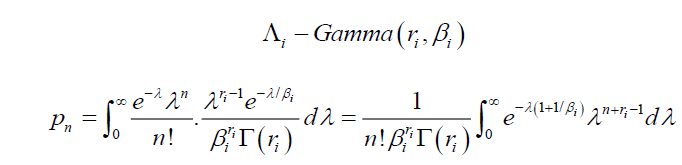
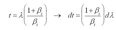
When allowing for uncertainty in default rates by assuming that ?i follows Gamma distribution, the resulting frequency distribution becomes a Poisson Mixture type called Negative Binominal. For each sector i, parameter λ of the Poisson distribution can be treated as an outcome of the random variable , which could be either continuous or discrete. In particular, we let the risk parameters to reflect heterogeneous risks. This is practically useful because not all individual lenders or individual bonds in the same rating category are exactly the same even though they may appear to be so.

When we allow λ varying across individual lenders or individual bonds, λ is unknown but follows some distribution. In other words, the true value of λ is unobservable. All we observe are the number of defaults. Thus, there is an uncertainty about the parameter.

Let u( λ) be the probability density function of and U(λ) be the cumulative density function of . The probability that exactly n defaults will occur can be written as the expected value (with respect to the distribution of ) of the same probability conditional on

If we look a little closer, the negative binomial distribution is indeed a mixture of the Poisson distribution and the Gamma distribution. To see this, let

Recall that

Let

and 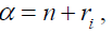then

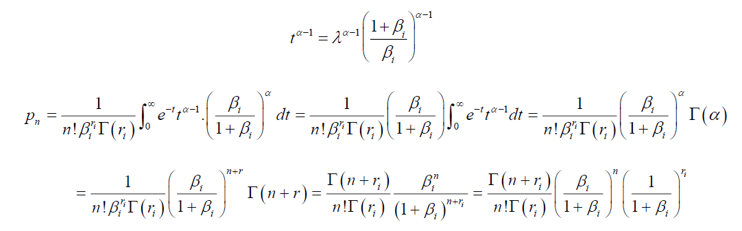
This is a probability density function of the Negative Binomial distribution with parameters Therefore, when allowing for uncertainty in default rates, the number of default for each sector follows Negative Binomial distribution.

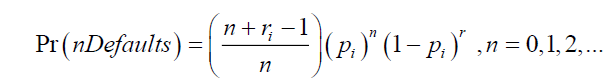
Let N_i be a random variable of the number of default in sector i. Then, N_i is assumed to follow Negative Binomial distribution with two parameters . For each sector i, the probability density function of N_i is represented by the following formula.

Where 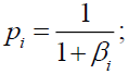and thus, 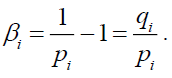The mean and variance of number of defaults for each sector i can be calculated as follow:

Since , the Negative Binomial distribution has its variance larger than its mean, which is more appealing in practice. However, unlike Poisson distribution, the summation of independent Negative Binomial random variable will not have a Negative Binomial distribution. Therefore, the default event distribution for the whole portfolio is not Negative Binomial, but can be represented by the following probability generating function.

Where, m is the number of sectors in the portfolio.

To surpass from default event to aggregate default loss distribution, the assumption on the individual loss distribution is needed. In this paper, we assume that the amount of credit loss has a gamma distribution. For each sector, the probability generating function of the aggregate loss random variable, X_i , can be derived from the probability generating functions of two random variables for default event and credit loss exposure, represented by N_i and X_i as follow:

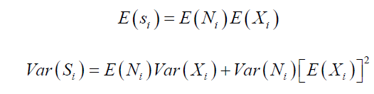
The mean and variance of aggregate loss random variable for each sector i can be obtained from the first two moments.

If each individual exposure X_i is represented by multiples of a monetary unit L, rounded to the nearest integer, the severity distribution will be defined on 0,1,2,…, n. Depending on the initial choice of L, a number of obligors will fall into the same category or band for the total number of n bands.

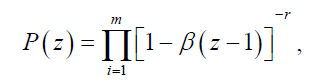
For each sector i, the number of default has the Negative Binomial distribution. Since the Negative Binomial distribution is a member of the (a, b, 0) class, the frequency distribution,π _k satisfies

Using the recursive method, we can obtain the following result of probability density function of aggregate loss for each sector i.

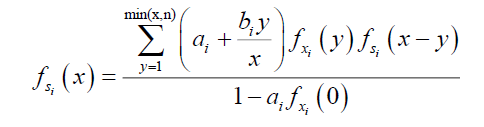
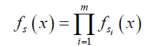
Because sectors are independent, the probability density function of aggregate loss for the whole portfolio can be written down as a product over the sectors.

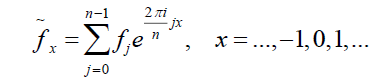
Alternatively, the aggregate loss distribution can also be calculated using Fast Fourier Transform (FFT). The FFT is an algorithm that can invert characteristic functions to obtain densities of discrete random variables. For any continuous function, the Fourier Transform or the characteristics function of x is defined by

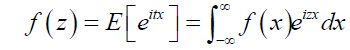
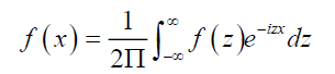
Where i is an imaginary unit, . The original density function, which is a real value, can be recovered from its Fourier Transform as

When X is a discrete random variable, which is the case of banding treatment in this paper, the discrete Fourier Transform becomes a simplified mapping of a vector of n values of real numbers to a vector of n values of complex numbers. The discrete Fourier Transform is defined by

Let aggregate loss of N individuals defaulted on loans represented by S. The Fourier Transform of S is derived by applying a probability generating function of N to That is,

The inverse FFT can be applied to recover the original distribution function of aggregate loss.

Melchiori (2004) proves that three approaches-Credit Risk recurrence relation, Panjer’s recursive formula and Fast Fourier Transform (FFT)-can provide the same result of aggregate loss distribution.

Data

Accounting data of major banks were retrieved from Nikkei NEEDS-Financial Quest database for the period of 2000 to 2015. Since this paper focuses on the effect of megabank mergers on credit risk, the sample drawn include only city banks and one remaining long-term credit bank, the Industrial Bank of Japan. Since two of the three long-term credit banks, the Long-Term Credit Bank of Japan and Nippon Credit Bank, became bankrupt during the study period, they were excluded from our study. The only remaining long-term credit bank, the Industrial Bank of Japan, merged with two city banks to form Mizuho Bank and Mizuho Corporate Bank.

Table 1 shows the number of city banks declining from 9 banks in 2000 to 4 remaining city banks in 2016², which include Mizuho bank, Sumitomo-Mitsui Banking Corporation (SMBC), Bank of Tokyo-Mitsubishi-UFJ and Resona Bank.

Table 1 : Number Of City Banks And Merger Events
Year	Number of City Banks	Merger Events
2001	9	Sakura Bank and Sumitomo Bank merged in April, 2001, to form Sumitomo Mitsui Banking Corporation.
2002	7	Mizuho Bank is a formed by the merger of the Dai-Ichi Kangyo Bank, the retail operations of Fuji Bank and Industrial Bank of Japan in April 2002.
		UFJ Bank is a merged bank between Sanwa Bank and Tokai Bank in January, 2002.
2003	6	On March 1, 2003, Resona Bank began its operation following the merger of Daiwa Bank with branches of the former Asahi Bank.
2006	5	On January 1, 2006, the Bank of Tokyo-Mitsubishi merged with UFJ Bank to form the Bank of Tokyo-Mitsubishi-UFJ.
2013	4	On July 1, 2013, Mizuho Bank and Mizuho Corporate Bank merged and began operating as the new Mizuho Bank.

A brief background of the establishment of each of the four remaining city banks is provided below.

Mizuho Bank, Ltd.

Mizuho Bank is a formed by the merger of the Dai-Ichi Kangyo Bank, the retail operations of Fuji Bank and Industrial Bank of Japan in April 2002. Mizuho Bank focuses on retail baking with 515 branches in every prefecture in Japan. Dai-Ichi Bank, the first bank ever to be established in Japan, merged with and the Nippon Kangyo Bank in 1971, creating the Dai-Ichi Kangyo Bank. Fuji Bank was formally known as Yasuda Bank. The name was changed after the World War II in 1941.

Mizuho Bank is a corporate and investment banking subsidiary of Mizuho Financial Group, the second largest financial services companies in Japan and one of the three Japanese megabanks, along with Mitsubishi UFJ Financial Group and Sumitomo Mitsui Financial Group. It was created by a transfer of corporate and investment banking divisions of Dai-Ichi Kangyo Bank and Fuji Bank to Industrial Bank of Japan.

On July 1, 2013, Mizuho Bank and Mizuho Corporate Bank merged and began operating as the new Mizuho Bank.

Bank of Tokyo-Mitsubishi-UFJ

In April 1996, the Bank of Tokyo and Mitsubishi Bank merged to form the Bank of Tokyo-Mitsubishi. UFJ Bank is a merged bank between Sanwa Bank and Tokai Bank in January, 2002. On January 1, 2006, the Bank of Tokyo-Mitsubishi merged with UFJ Bank to form the Bank of Tokyo-Mitsubishi-UFJ.

Sumitomo Mitsui Banking Corporation

A long history of the Sakura Bank started in 1876, when Mitsui family founded the first private bank in Japan, the Mitsui Bank. It merged with Dai-Ichi Bank to form the Teikuko Bank in 1943, but changed the name back to Mitsui Bank in 1954. It merged with Toto Bank in 1968 and again with Taiyo Kobe Bank in 1990. In 1992, Mitsui Bank was renamed Sakura Bank. Sakura Bank and Sumitomo Bank merged in April, 2001, to form Sumitomo Mitsui Banking Corporation with the total capital stock of 1,276.7 billion yen. It then failed to take over UFJ Bank, that later merged with the Bank of Tokyo-Mitsubishi. Mitsui Banking Corporation is currently the third largest bank in Japan.

Resona Bank

On March 1, 2003, Resona Bank began its operation following the merger of Daiwa Bank with branches of the former Asahi Bank remaining after the split-off of Asahi Bank branches operating in Saitama prefecture.

Results

Total assets of all city banks are accounted for more than 50% of all banks in Japan. City banks have total deposit of about 49% of the total deposits in Japanese Banking system. A loan portfolio of each bank can be created using the detail information of corporate borrowing from financial institutions. We can identify bad loan by using the detail information of the non-performing loans for all city banks and the Industrial Bank of Japan during the study period.

Balance of Non-Accrual Delinquent Loans is the balance of loans considered delinquent but has not as yet been written off as bad debts is placed on a non-accrual basis. That is, even though the loans still remain on the book, the bank stops accruing interest income on this loan. These loans could still be in the process of being restructured or renegotiated.

We apply Fast Fourier Transform method to data of detailed loan and detailed NPL by sector from Nikkei database to calculate the credit VaR of the banks before and after mergers. Credit reserve is subtracted from credit VaR to derive additional economic capital that the bank should hold against a given portfolio. The outcome of additional capital is then divided by risk-adjusted assets to represent required capital adequacy ratios shown in Table 2.

Table 2 : Required Capital Adequacy Ratios Based On Credit Var
Year	Before merger		After merger
2001	Sakura Bank	Sumitomo Bank	Sumitomo Mitsui Banking Corporation
	11.91	11.87	10.46
2002	Dai-Ichi Kangyo Bank	Industrial Bank of Japan	Mizuho Bank
	12.45	14.53	12.48
	Sanwa Bank	Tokai Bank	UFJ Bank
	13.48	12.24	11.24
2003	Daiwa Bank	Asahi Bank	Resona Bank
	11.73	11.41	10.17
2006	Bank of Tokyo-Mitsubishi	UFJ Bank	Bank of Tokyo-Mitsubishi-UFJ
	13.44	10.24	9.97
2013	Mizuho Bank	Mizuho Corporate Bank	Mizuho Bank
	12.35	15.33	11.49

In all six bank merger events during our study period, the merged banks benefit from lower capital requirement as a percentage of risk-adjusted assets. These results provide solid evidence that credit risk diversification could be one of the main incentives for Japanese bank mergers.

Conclusion

Japanese banks have undergone a major consolidation. The government encouraged the mergers of weakened banks and the purchase of nationalized insolvent bank. A consolidation of an efficient bank with an inefficient bank does not create an efficient bank. Moreover, a merger of both inefficient banks would not lead to a more efficient bank either. Nonetheless, mergers still take place as part of an effort to increase comparative advantage in banking system in Japan. Thus, incentives for bank consolidation in Japan might not be solely for efficiency improvement, but more toward lower credit risk of their combined loan portfolio.

This paper proposes an actuarial model to prove that credit risk diversification is an incentive for Japanese bank mergers. An advantage of using an actuarial model is that it is not subject to precision problems that can arise from simulation-based approach. Actuarial methods are increasingly used and accepted by auditors and regulators as a means to determine a bank’s reserve. Similar to insurance business, expected loss is an important indicator determining the adequacy of product pricing model.

In this paper, credit risk is defined as potential future credit loss due to credit events and credit VaR as the maximum possible loss for a given position of a portfolio given a certain confidence level over a specified time horizon. There are two distinct definitions of credit losses: Expected losses and unexpected losses. The unexpected loss is referred to as the difference between maximum possible loss and expected loss. Indeed, credit VaR is the unexpected loss of the loan portfolio and represents the additional economic capital that the bank should hold against a given portfolio above the level of credit reserves because the actual credit losses in any given period could be significantly higher than the expected level.

Based on actuarial techniques, an aggregate loss distribution is generated from credit loss frequency and severity distributions. Allowing for uncertainty in default rates, the number of default for each sector follows Negative Binomial distribution. The aggregate loss distribution based on accounting data of city banks from Nikkei NEEDS-Financial Quest database, for the period of 2000 to 2015, are then calculated using Fast Fourier Transform (FFT). Credit VaR before and after the merger events were calculated. The expected credit loss is then subtracted from credit VaR to measure economic capital requirement as a percentage of risk weighted assets. There were six bank merger events during our study period, the merged banks benefit from lower capital requirement as a percentage of risk-adjusted assets. These results of required capital adequacy ratios provide strong evidence that credit risk diversification could be one of the main incentives for Japanese bank mergers.

Endnotes

1. Published Land Prices (2004), Ministry of Land, Infrastructure and Transport, Japan.

2. List of Licensed Financial Institutions, City Banks, Financial Services Agency (as of October 27, 2016).

References

1. Batten, J.A. & Vo, X.V. (2016). Bank risk shifting and diversification in an emerging market. Risk Management, 18(4), 217-235.
2. Chalikias, M., Lalou, P. & Skordoulis, M. (2016). Modelling advertising expenditures using differential equations: The case of an oligopoly data set. International Journal of Applied Mathematics and Statistics, 55(2), 23-31.
3. Chalikias, M., Lalou, P. & Skordoulis, M. (2016). Modelling a bank data set using differential equations: The case of the Greek banking sector. Proceedings of 5th International Symposium and 27th National Conference of HEL.O.R.S on Operation Research, 113-116.
4. Casu, B., Dontis?Charitos, P., Staikouras, S. & Williams, J. (2016). Diversification, size and risk: The case of bank acquisitions of nonbank financial firms. European Financial Management, 22(2), 235-275.
5. Credit Suisse First Boston. (1997). A credit risk management framework documentation. Credit risk.
6. Doumpos, M., Gaganis, C. & Pasiouras, F. (2016). Bank diversification and overall financial strength: International evidence. Financial Markets, Institutions & Instruments, 25, 169-213.
7. Drake, L. & Hall, M.J.B. (2000). Efficiency in Japanese banking: An empirical analysis. Economic Research Paper, Loughborough University.
8. Filson, D. & Olfati, S. (2014). The impacts of Gramm-leach-Bliley bank diversification on value and risk. Journal of Banking & Finance, 41, 209-221.
9. Goetz, M.R., Laeven, L. & Levine, R. (2016). Does the geographic expansion of banks reduce risk? Journal of Financial Economics, 120(2), 346-362.
10. Gordy, M. (2000). A comparative anatomy of credit risk models. Journal of Banking and Finance, 24(1-2), 119-149.
11. Gulamhussen, M.A., Pinheiro, C. & Pozzolo, A.F. (2014). International diversification and risk of multinational banks: Evidence from the pre-crisis period. Journal of Financial Stability, 13, 30-43.
12. Harada, K. (2005). Did efficiency improve megamergers in Japanese banking sector? Working Paper CNAEC Research Series, Korea Institute for International Economic Policy.
13. Morgan, J.P. (1997). Credit metrics-technical documentation. New York: J.P. Morgan.
14. Kealhofer. (1995). Portfolio management of default risk, proprietary documentation. San Francisco: KMV Corporation.
15. McKinsey. (1998). Credit portfolio view approach and user’s documentation. New York: McKinsey & Company.
16. Melchiori, M.R. (2004). Credit risk by fast Fourier transforms. e-Journal.
17. Ono, A. (2006). The role of credit scoring in small business lending, financial information infrastructure and SME finance. ADB Institute.
18. Saunders, A. & Allen, L. (2002). Credit risk measurement: New approaches to value at risk and other paradigms (Second Edition). John Wiley & Sons, New York.
19. Shimizu, T. & Shiratsuka, S. (2000). The credit risk of Japanese banks during the bubble period: A pilot study of macro stress simulation. IMES Discussion Paper Series.
20. Wilson, T. (1997a). Measuring and managing credit portfolio risk: Modelling systematic risk. Journal of Lending and Credit Risk Management.
21. Wilson, T. (1997b). Measuring and managing credit portfolio risk: Tabulating loss distributions. Journal of Lending and Credit Risk Management.
22. Wilson, T. (1997c). Portfolio credit risk. Risk Magazine.
23. Wilson, T. (1997d). Portfolio credit risk. Risk Magazine.