Keywords

Digital Logistics, Economic and Mathematical Models, Digital Twins

Introduction

The construction, improvement and development of any transport system is aimed primarily at meeting the demand for the transportation of goods between regions of production and consumption through transit zones, countries and continents. Thus, the volume of the expected freight traffic is the initial information for the design of the throughput of main lines, transshipment complexes and vehicles. But transport by its nature is more multifaceted, its activities are associated with all branches of production and the lives of hundreds of millions of people acting as consumers of goods and transport services (Barykin et al., 2021). Therefore, it is especially difficult to foresee the future of communication routes. By virtue of which, one or another current state of the transport system in the future cannot be determined based only on the principles of determinism (Sacks et al., 2020).

The prospective state of transport also cannot be determined statistically, since the development of transport is not a formalized process, constantly accompanied by qualitative changes in its infrastructure due to uneven congestion and a change in orientation, both of individual elements and of the transport system as a whole (Atzori, Iera & Morabito, 2010; Shen & Liu, 2011).

Thus, a holistic picture of the interaction of nodes in a logistics network with an analysis of the current state and potential outcomes can only be provided by the system of Digital Twins (DT), which is based on continuous analysis of statistical indicators, analysis of current indices of the state of elements and variable series of potential outcomes (Kritzinger et al., 2018).

Theoretical Foundation

A Conceptual Apparatus

Due to their high cost, the lengths of the transport network, the location of cargo transshipment points, as well as such operational characteristics of transport as the average speed of delivery of goods and the ratio of loaded and empty runs along the track sections, are more inertial, due to their high cost. Less inertial due to the gradual renewal of the carrying capacity of means of transport (Zhang et al., 2019; AnyLogistix, 2020).

With the expansion of the forecasting horizon, the assessment of the prospects for the congestion of transport modes becomes less certain, since the likelihood of changes of a fundamental nature increases, for example, the construction of new sea terminals, regional centers for the consolidation and unbundling of cargo consignments, on the basis of which new routes for the transportation of goods are laid (Balaban, 2019).

To assess the strategy for the future development of the industry, economic forecasting is used, which makes it possible to develop recommendations for making management decisions. Economic forecasts provide initial data on the basis of which it is possible to increase the validity of the organization of transport management (Borisoglebskaya et al., 2019).

In turn, already existing transport systems do not always fit into the mathematical models and concepts built on their basis, since each of these models describes only certain aspects of the transport system and sometimes within very narrow boundaries.

The most reliable idea of the possibilities and prospects of transport in general and its elements can only be provided by a complex application of various theoretical methods and concepts of quantitative and qualitative analysis, as well as taking into account the mutual influence of various factors (Krasnov et al., 2019). Here it is important to proceed from the fact that the development of transport is a constant progressive process, stretched out over a long period. Moreover, each subsequent stage of transport development is based on the achievements of the previous one. Thus, the development prospects are based on the previously achieved result, which in turn gives researchers the opportunity to predict the new quantitative and qualitative state of transport networks (Barykin et al., 2020).

A Digital Twin (DT) is a virtual prototype of a real object, group of objects or processes. A digital twin is a complex software product created using analytical and statistical data, simulation models, a system of variable rad and mathematical forecasting models. The digital twin is not limited to collecting data obtained during the development and production of a product, it continues to collect and analyze data throughout the entire lifecycle of a real object, including using numerous IoT sensors (Aranguren et al., 2018).

Based on the definition of the Digital, we conclude that in the conditions of decision-making based on the analysis of stochastic information and changing indicators, the use of methods of economic and mathematical modeling and analysis is not only justified, but also necessary (Campbell & O’Kelly, 2012).

Econometric models are systems of interrelated equations and are used to quantify the parameters of economic processes and phenomena.

Economic processes develop over time; therefore, an important place in econometrics is occupied by the analysis and forecasting of time series, including multidimensional ones. At the same time, in some tasks, more attention is paid to the study of trends (average values, mathematical expectations), for example, when analyzing the dynamics of transportation prices (Fu, Chen & Xue, 2018).

Econometric methods are needed to assess the parameters of economic and mathematical models of logistics. A striking example of the use of econometric methods is the analysis of the dynamics of prices and traffic volume (Gruchmann, Melkonyan & Krumme, 2018).

Almost any field of economics deals with the statistical analysis of empirical data, and therefore has certain econometric methods in its toolbox.

With the help of econometric methods, it is necessary to evaluate various quantities and dependencies used in the construction of simulation models of processes.

Multivariate Predictive Functions

Each predicted indicator ?t (t=1,2 ..., n) can be considered not only as a function of one factor-argument, but also on several:

- in the form of a linear multivariate model:

where a0, aj are the coefficients of the model at j=1, 2,…, k;

?jt - factors-arguments influencing the predicted indicator ?t, at j=1, 2,…, m; t=1,2, ..., n;

- in the form of a nonlinear multivariate model (power type):

which is converted to linear by taking the logarithm. More complex types of nonlinear multivariate models are rarely used in forecasting and planning practice.

Coefficients a0, aj in models of type (1) and (2) are determined using the least squares method from a system of normal equations, which are partial derivatives with respect to a0, and aj equal to zero:

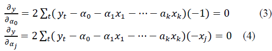
As a result of solving this system of equations, such a0 and aj are found for which tends to zero.

The factors-arguments must meet the following conditions: first, have a quantitative measurement and be reflected in the reports or, at least, be determined on the basis of a special analysis of the reported data; secondly, to have prospective estimates of values for the forecast period; third, the number of factors included in the model should be three times less than the number of data in the series; fourth, to be linearly independent (Pilipenko et al., 2019).

Factors are considered dependent (multicollinear) if the linear (pairwise) correlation coefficient of two factors is more than 0.8. Of these, the model is left with the one that has the highest correlation coefficient with the function y.

The optimal number of factor-arguments can be established using the so-called exclusion method.

The type model includes all possible factors that satisfy the above conditions and build this model. For each j-th factor-argument, the Student's estimates are found using the formula. The smallest value of the estimate mint a1 is selected and compared with the tabular value - tp at (n-k-1) - degrees of freedom and the selected significance level p (usually p=0.05 or 5%). If the minimum of the calculated estimates is ta> tp, then the model is left as it is. If tap, then the a1 factor is excluded from the model as insignificant. Then, with the remaining factors, a new model is built, a new value of the Student's estimates is determined, the minimum of them is found, etc. until all significant factors remain in the model.

The tightness of relationships between the function and the factor-arguments can be established using the square of the multiple correlation coefficients:

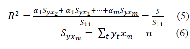
The squared coefficient of multiple correlation shows how much of the total dispersion of the dependent variable can be explained by a function of the form (5) or form (6).

The statistical reliability of a multivariate regression model (or coefficient of determination) is established using Fisher's test:

where n - is the number of data;

m - is the number of factor-arguments in the model;

R2 is the square of the multiple correlation coefficient.

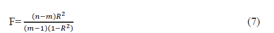
If the calculated value of the Fisher criterion exceeds the tabular value for (n-m) and (m-1) degrees of freedom and the accepted p - significance level, then the model is recognized as statistically reliable and significant. The multivariate regression model can be used to predict no more than a three-year lead period. Forecast errors are determined by the formulas.

Exponential Smoothing Method

The essence of this method lies in the fact that the forecast of expected values (volumes, sales, etc.) is determined by the weighted average values of the current period and smoothed values made in the previous one. This process continues back to the beginning of the time series and is a simple exponential model for time series with a steady trend and small (independent) periodic fluctuations (Bogers et al., 2019).

For many time series (indicators), there is an obvious pattern of periodicity and randomness. Therefore, the simple exponential model expands to include the last two components.

With a Steady Trend

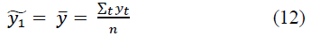
Let the ironed value at time t be determined by the recurrent formula:

where yt - is the actual value at time t;

a - is the smoothing parameter, determined by the formula Then the smoothed value at time (t-1) is:

Substituting into the formula, we get:

Continuing this process, the forecast can be expressed in terms of the past values of the time series:

where L is the prediction period, but not more than three to five years.

For t=1,2, ..., n, the smoothed values at time t are determined by the formula. For the same time period, the standard deviation and the coefficient of variation are determined to assess the accuracy of the selected smoothing parameter.

For t=1

If the coefficient of variation exceeds 10%, then it is necessary to change the smoothing interval, and, consequently, the smoothing parameter.

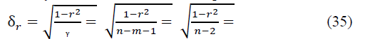
For, ..., n, the forecasts at time t are determined by the formula for assessing the prediction accuracy by the standard deviation and the coefficient of variation.

When t=n+1, n+2, …, the forecasts of this indicator are determined accordingly, under the assumption that the current value at the time t=n+1 coincides with the forecast at the time t=n.

With a Periodic Component

Let be the smoothed value at time t taking into account the periodic component. The periodicity coincides with the prediction period. In practice, annual or monthly changes are usually considered. Then the estimate of the smoothed value will be written as follows:

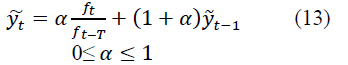
where ft-T is the estimate of the periodic component in the previous period; T - is the length of the period.

At time t, the periodic component is determined by the formula:

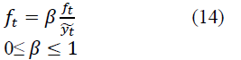
The weight parameters α and β are selected either taking into account the current values of, or taking into account the past values of their optimal values are set at the minimum standard deviation.

The forecast of the expected values for evaluating the selected parameters α and β can be determined in a multiplicative way by the formula:

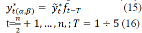
At t=n+1, n+2, ..., N, the actual forecasts are determined by the formula:

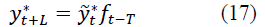
Where yt* - is the forecast of the smoothed value determined by the formula.

c) With periodic and random components

Let the estimate of the smoothed value, taking into account the periodic and random components, have the form:

where εt-1 is the estimate of the random component at the moment of time (t-1), the current value of εt is determined by the formula:

where γ is the smoothing parameter for the random component 0≤ γ ≤ 1,.

The forecast of the expected values for the assessment of the selected parameters α, β and γ can be obtained by the formula:

where T is the prediction period, T=1, 2, ..., 5;

, …, n.

At t=n+1, n+2, ..., N, the actual forecasts are determined by the formula:

d) Autoregressive transformation method

Its essence lies in building a model based on deviations of the values of the time series from the values aligned along the trend. Let these deviations represent random fluctuations in the time series at each moment of time t:

Then, for the random variable εt, an auto regression model can be constructed, i.e., linear regression model for residuals of time series values. These random variables are distributed with an average value of 0 and finite dispersion (variance) and obey the law of the 1st order stochastic linear difference level with constant coefficients (Markov process), that is:

where εt-1 is the time series of the random component shifted by one step, t=1, 2,…, n. Using formulas of the form (23), we determine b0 and b1, we obtain:

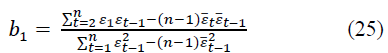
Where and - are the average values for the given time series and shifted by one step, respectively.

The predicted values of the random component are determined by the formula:

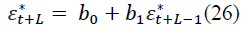
L=1, 2, …

At L=1, at L=2, 3,… the formula is valid.

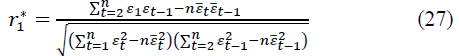
Determine the autocorrelation coefficient r2 using the formula of the pair correlation coefficient. Then the autocorrelation coefficient for the 1st order autoregressive model is:

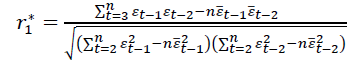
Then we compose the 2nd order autoregressive model:

where εt-2 is the time series of the random component, shifted by two steps, for t=1, 2,…, n.

Coefficients b0, b1, b2 are found using the least squares method from the system of normal equations.

We find:

If, r*1>r*2 then the random component follows the law of the 1st order linear difference equation, and the predictions are determined by the formula. If, r*1>r*2 then, a linear difference equation of the 3rd order is calculated r*3, etc. These calculations continue until , at τ=1,2, ..., n/2. An autoregressive model of (τ-1) order is chosen. The estimation of the accuracy and reliability of the autoregressive model is determined by the standard deviation and the coefficient of variation.

Correlation-Regression Analysis

This method contains two of its components - correlation analysis and regression analysis. Correlation analysis is a quantitative method for determining the closeness and direction of the relationship between sample variables. Regression analysis is a quantitative method for determining the type of mathematical function in a causal relationship between variables.

Linear Correlation

This correlation characterizes the linear relationship in the variation of variables. It can be paired (two correlated variables) or multiple (more than two variables), direct or inverse - positive or negative, when the variables vary in the same or different directions, respectively.

If the variables are quantitative and equivalent in their independent observations with their total number n, then the most important empirical measures of the tightness of their linear relationship are the coefficient of direct correlation of the signs of the Austrian psychologist (Fechner, 1801-1887) and the coefficients of pair, pure (private) and multiple (cumulative) correlation of English statistician-biometrics (Pearson, 1857-1936).

The coefficient of pair correlation of Fechner's signs determines the consistency of directions in individual deviations of the variables x and y from their means. It is equal to the ratio of the difference between the sums of coinciding (C) and non-coinciding (H) pairs of signs in deviations and to the sum of these sums:

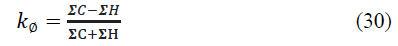
The Kφ value varies from -1 to +1. The summation is carried out over observations that are not indicated in the amounts for the sake of simplicity. If anyone deviation or then it is not included in the calculation. If both deviations are zero at once: then such a case is considered to be the same in signs and is part of C.

Coefficients of pairwise, pure (partial) and multiple (cumulative) linear Pearson correlation, in contrast to the Fechner coefficient, take into account not only the signs, but also the magnitudes of the deviations of the variables. Different methods are used to calculate them. So, according to the method of direct counting on ungrouped data, the Pearson pair correlation coefficient has the form:

This coefficient also varies from -1 to +1. If there are several variables, the Pearson multiple (cumulative) linear correlation coefficient is calculated. For three variables x, y, z, it has the form like:

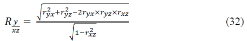
This coefficient varies from 0 to 1. If we eliminate (completely exclude or fix at a constant level) the influence of z on x and y, then their “general” relationship will turn into “pure”, forming a pure (private) Pearson linear correlation coefficient:

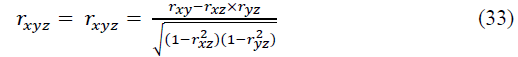
This coefficient ranges from -1 to +1. The squares of the correlation coefficients (31) - (33) are called the coefficients (indices) of determination - respectively, pair, pure (partial), multiple (total:

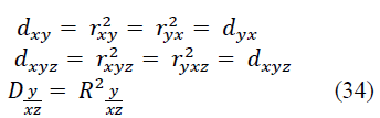
Each of the coefficients of determination varies from 0 to 1 and estimates the degree of variational certainty in the linear relationship of variables, showing the proportion of variation of one variable (y) due to the variation of the other (others) - x and y. The multidimensional case of more than three variables is not considered here.

According to the developments of the English statistician R.E. Fisher (1890-1962), the statistical significance of the paired and pure (private) Pearson correlation coefficients is checked if their distribution is normal, based on the t-distribution of the English statistician V.S. Gosset (pseudonym "Student"; 1876-1937) with a given level of probabilistic significance and available degrees of freedom, where m - is the number of links (factor variables). For the paired coefficient rxy, we have its root-mean-square error and the actual value of the Student's t-test:

For a pure correlation coefficient rxyz, when calculating it, instead of (n-2), one should take (n-3), since in this case, there is m=2 (two factorial variables x and z). For a large number n> 100, instead of (n-2) or (n-3) in (6), you can take n, neglecting the accuracy of the calculation.

If tr> t, then the coefficient of pair correlation - general or pure - is statistically significant, and for tr ≤ ttabl. - insignificant.

The significance of the multiple correlation coefficient R is checked by F - Fisher's criterion by calculating its actual value

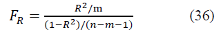
At FR> Ftab. the coefficient R is considered significant with a given level of significance a and the available degrees of freedom and , and at Fr ≤ Ftabl - insignificant.

In large-scale aggregates n> 100, to assess the significance of all Pearson's coefficients, instead of the t and F criteria, the normal distribution law is applied directly (the tabulated Laplace-Sheppard function). Finally, if Pearson's coefficients do not obey the normal law, then Fisher's Z test - is used as a criterion for their significance, which is not considered here.

Results

Based on the Above Examples, the Following Conclusions can be drawn

A forecast is understood as a system of scientifically grounded ideas about the possible states of an object in the future, about alternative ways of its development. The forecast expresses foresight at the level of a specific applied theory, at the same time, the forecast is ambiguous and has a probabilistic and multivariate character. The process of developing a forecast is called forecasting.

The most important component of the macro-forecasting methodology is the methodological principles, which are understood as the initial provisions, the fundamental rules for the formation and substantiation of plans and forecasts. They provide purposefulness, integrity, a certain structure and logic of the developed plans and forecasts (Tuegel et al., 2011; Weyer et al., 2016).

Forecasting methods are methods, techniques with the help of which the development and justification of plans and forecasts is ensured.

There are a lot of such forecasting methods and models, and each of them has its own certain accuracy, based on certain factors.

Thus, we can conclude that in order to create the most accurate and universal system of distribution paths in the system of digital twins of logistics networks in general, and hubs in particular, it is necessary to combine various methods of mathematical and economic forecasting into a single system (Krasnov et al., 2019).

If we take as a basis the understanding that any forecasting is based on the theory of probability, taking into account the influence of external factors on the share of a particular probabilistic outcome, then in a simplified form the forecasting scheme can be visualized as follows (Figure 1):

Based on this, the system of variable outcomes based on several mathematical models can be schematically expressed in (Figure 2):

Summing up, it is possible to schematically depict a universal system of distribution paths in a system of digital twins in the form of a mathematical transport problem with multifactor forecasting models in each of the blocks (hubs) (Figure 3):

Discussion

Considering digital twins in logistics, it is worth noting that in this sector, the factor of predicting freight flows and seasonal characteristics within transportation networks is of the greatest importance. The creation of digital twins in this sector is the most difficult and time-consuming task, the solution of which has enormous potential in terms of optimizing all logistics networks in general (Tekinerdogan & Verdouw, 2020).

Conclusion

According to the study, it can be noted that the digital twin has enormous potential and is used in the daily operation of various networks. The internal structure of the DT is built on the basis of multiple, multifactorial mathematical intertwining models. It is this base, when automating processes, that allows you to analyze all possible factors of influence on transportation within the network and processes within logistics hubs (Christensen, Olesen & Kjær, 2005).

The article presents the concept of digital twins and econometric models as the basis for their construction. Analyzed and described the mathematical modeling of the analysis and planning system in logistics networks.

This study analyzes various econometric methods of analysis and forecasting, describes their features and possible results obtained when using them.

It should be borne in mind that each mathematical model has its own approach, and certain factors are analyzed to obtain specific information. These models are not completely interchangeable, which means that in order to obtain comprehensive data for choosing the optimal sequence of actions, mutual integration of mathematical models is necessary (Yun, Kim & Yan, 2020).

References

1. AnyLogistix. (2020). Supply chain digital twins. Definition, the problems they solve, and how to develop them. Available at: https://www.anylogistix.com/supply-chain-digital-twins/.
2. Aranguren, M.F., Villar, C.K.K., Ojeda, A.M., & Giacomoni. M.H. (2018). Simulation-optimization approach for the logistics network design of biomass co-firing with coal at power plants. Sustainability (Switzerland), 10(11).
3. Atzori, L., Iera, A., & Morabito, G. (2010). The internet of things: A survey. Computer Networks. Elsevier B.V. 54(15), 2787–2805.
4. Balaban, O.R. (2019). Approximation of evolutionary differential systems with distributed parameters on the network and moment methods. Modeling, Optimization and Information Technology” (“MOIT”), 7(3). Available at: http://moit.vivt.ru/.
5. Barykin, S.Y. (2021). Developing the physical distribution digital twin model within the trade network. Academy of Strategic Management Journal, 20(1), 1–24. Available at: https://www.abacademies.org/articles/developing-the-physical-distribution-digital-twin-model-within-the-trade-network.pdf.
6. Barykin, S.Y., Bochkarev, A.A., Kalinina, O.V., & Yadykin, V.K. (2020). Concept for a supply chain digital twin. International Journal of Mathematical, Engineering and Management Sciences, 5(6), 1498–1515.
7. Bogers, M., Chesbrough, H., Heaton, S., & Teece, D.J. (2019). Strategic management of open innovation: A dynamic capabilities perspective. California Management Review, 62(1), 77–94.
8. Borisoglebskaya, L.N., Provotorova, E.N., Sergeev, S.M., & Khudyakov, A.P. (2019). Automated storage and retrieval system for Industry 4.0 concept. IOP Conference Series: Materials Science and Engineering, 537(3), 0–6.
9. Campbell, J.F., & O’Kelly, M.E. (2012). Twenty-five years of hub location research. Transportation Science, 46(2), 153–169.
10. Christensen, J.F., Olesen, M.H., & Kjær, J.S. (2005). The industrial dynamics of open innovation - Evidence from the transformation of consumer electronics. Research Policy, 34(10), 1533–1549.
11. Fu, X.M., Chen, H.X., & Xue, Z.K. (2018). Construction of the belt and road trade cooperation network from the multi-distances perspective. Sustainability (Switzerland), 10(5).
12. Gruchmann, T., Melkonyan, A., & Krumme, K. (2018). Logistics business transformation for sustainability: Assessing the role of the lead sustainability service provider (6PL). Logistics, 2(4), 25.
13. Krasnov, S., Sergeev, S., Titov, A., & Zotova Y. (2019). Modelling of digital communication surfaces for products and services promotion. IOP Conference Series: Materials Science and Engineering, 497(1).
14. Krasnov, S., Sergeev, S., Zotova, E., & Grashchenko, N. (2019). Algorithm of optimal management for the efficient use of energy resources. E3S Web of Conferences, 110.
15. Kritzinger, W., Karner, M., Traar, G., Henjes, J., & Sihn, W. (2018). Digital twin in manufacturing: A categorical literature review and classification. IFAC-PapersOnLine. Elsevier B.V, 51(11), 1016–1022. Available at: https://doi.org/10.1016/j.ifacol.2018.08.474.
16. Pilipenko, O.V., Provotorova, E.N., Sergeev, S.M., & Rodionov, O.V. (2019). Automation engineering of adaptive industrial warehouse. Journal of Physics, Conference Series, 1399(4).
17. Sacks, R., Brilakis, I., Pikas, E., Xie, H.S., & Girolami, M. (2020). Construction with digital twin information systems. Data-Centric Engineering, 1.
18. Shen, G., & Liu, B. (2011). The visions, technologies, applications and security issues of internet of things. 2011 International Conference on E-Business and E-Government, ICEE2011 - Proceedings. IEEE, 1867–1870.
19. Tekinerdogan, B., & Verdouw, C. (2020). Systems architecture design pattern catalog for developing digital twins. Sensors (Switzerland), 20(18), 1–20.
20. Tuegel, E.J., Ingraffea, A.R., Eason, T.G., & Spottswood, S.M. (2011). Reengineering aircraft structural life prediction using a digital twin. International Journal of Aerospace Engineering.
21. Weyer, S., Meyer, T., Ohmer, M., Gorecky, D., & Zühlke, D. (2016). Future modeling and simulation of CPS-based factories: An Example from the Automotive Industry. IFAC-PapersOnLine. Elsevier B.V, 49(31), 97–102. Available at: http://dx.doi.org/10.1016/j.ifacol.2016.12.168.
22. Yun, J.J., Kim, D., & Yan, M.R. (2020). Open innovation engineering—preliminary study on new entrance of technology to market. Electronics (Switzerland), 9(5), 1–10.
23. Zhang, C. (2019). A reconfigurable modeling approach for digital twin-based manufacturing system. Procedia CIRP. Elsevier B.V. 83, 118–125. Available at: https://doi.org/10.1016/j.procir.2019.03.141.