Research Article: 2019 Vol: 18 Issue: 6
Efficiency for Agro-Based Industrial Sub-Sector in Malaysia Using Data Envelopment Analysis (DEA)
Siti Marsila Mhd Ruslan, Universiti Malaysia Terengganu
Abstract
Keywords
Efficiency, Agro-Based Industry, DEA, BCC Model, CCR Model.
Introduction
Malaysia is a country that began to rise as an economic power in Southeast Asia. Throughout 2000 to 2008, its purchasing power parity has increased 4.7 times from 87.629 billion USD in 1990 to 412.302 billion USD in 2010. Among members of the Association of Southeast Asian Nations (ASEAN), Malaysia also emerged as the third country with largest income per capita, with 61% of the population is comprised of middle and high income groups (Ahmad & Rohana, 2006). Also, the development in manufacturing sector has provided a significant growth in maintaining the unemployment rate as low as 3.2% in 2007 and 3.3% in 2008 (Mat Nasir et al., 2007).
Nevertheless, behind the transformation of economic restructuring that Malaysia experienced in the 90’s until 2000’s, the agricultural sector is still being regarded as the most important sector due to its role as the sole food provider, as well as the inputs for manufacturing sector. Although the agricultural sector is seen as less impressive than the manufacturing sector, this sector has actually acted as the national saviour during the financial downturn in the late 1990s. Not only looking at its gross output contribution, the revenue through exports also increased during the era of currency depreciation (Mad Nasir et al., 2012; Wong, 2007). Therefore, in order to further develop this sector, the government has focused on improving the sector by introducing a business-oriented agricultural sector.
In the 9th Malaysia Plan (2006-2010), the agriculture sector has been expected to be the third largest engine for economic growth, which grow at an average rate of 5% per annum and with the inclusion of agro-based industries, the growth rate is expected to increase to 5.2% per annum (Yusof et al., 2006). Over the course of time, the growth of the agricultural sector was largely contributed by expansion by food commodities sub-sector which is projected to grow by 7.6% per annum besides the commodity sub-sector industry which is expected to expand by 3.2% per year (Yodfiatfinda et al., 2012).
Regarding to that, although the National Agricultural Policy (NAP) succeeded in increasing the output of the agricultural sector, however, it was seen as less successful in reducing the gap between the productivity of the labour force between the agricultural sector and the overall economy, especially in the manufacturing sector. The ratio of labour productivity in the agricultural and manufacturing sectors declined from 0.51 in 1985 to 0.49 in 1990 (Muzafar, 2006). Employment in the agricultural sector is said to be expected to contract at an average rate of 1.2% per annum to 1.3 million in 2010. However, labour productivity is expected to improve from RM15, 752 in 2005 to RM21, 2999 in 2010. For the period in between 2001 and 2005, the registered agricultural sector showed a growth rate of 2.4% (Yusof et al., 2006).
With the background of industrial sector, agro-based sectors are seen to be significant to economic growth due to its nature of capability in generating nation’s economy and income; not only on the production side but also through export taxes. Many foreign exchange earnings are seen through exports that involve with agricultural commodities and sector investments such as advancing the production output through infrastructure building and latest technologies.
The scope of this study focuses on seven sub-sectors of agro-based processing industry namely coconut oil manufacturing, palm oil manufacturing, chocolate production, coffee production, rubber production, rice production and wheat flour. In addition, this study is also expected to evaluate the effectiveness of the government's strategy towards the agricultural sector in the face of global financial crisis that took place in 1998, while taking account on the National Agricultural Policies (NAP).
Literature Review
It is undeniable that agricultural sector is a major engine sector in contributing to the Malaysian economy. Nevertheless, this sector had experience a downfall in its output during 1990s. For instance, in 1980 to 1990, the value added contribution of agricultural sector to the national Gross Domestic Product (GDP) had fell from 22.9-18.7% and further declined to 13.6% in 1995 (Murad et al., 2008 & 2009; Cho, 2011). In 1990, the pie share of employment in agricultural sector fall from 39.7% which recorded in 1980 to just 27.8%. In contrast, the manufacturing sector had increased its value added by 13.3% per year during 1991 to 1995, and by 1995, the sector had been contributing at 33.1% to GDP (Ministry of Agriculture and Agro-Based, n.d.).
Following to the trend and to spur the growth of agricultural sector, the First National Agricultural Policy was officiated in 1984 by the Ministry of Agriculture with a purpose to maximize income through optimal utilization of domestic resources and recovery of the sectors contribution to the overall economic development (Indrani et al., 2001; Matahir & Tuyon, 2013). The focus of the policy was mainly to increase farms’ productivity by selecting “profitable” crops and incorporating the most efficient technologies. Nonetheless, the First National Agricultural Policy was not successful in increasing income and overcoming productivity disparity between agricultural sector and the whole economy, particularly the manufacturing sector (Shobri et al., 2016; Shapira et al., 2006). Due to that scenario, an improvement in provision of adequate support services and infrastructure in agricultural production areas was needed, as to further boost the productivity in the sector. It is also foreseeable that productivity will also be surged through bigger application of the latest technology and knowledge-based production systems (Courtenay, 1987; Okposin et al., 1999).
Due to inevitable shortfalls and constant inefficiencies, the Second National Agricultural Policy (1992-1997) was introduced in 1998 and eventually followed by Second National Agricultural Policy (1992-1997). The new policy was aimed with an objective in sustaining the development towards a more dynamic agricultural sector, in a way that the growth has to be market-led, commercialized, efficient and competitive (Rasiah & Shari, 2001). The sole aim was to boost up income through efficient utilization of resources. Nevertheless, the objectives of this new policy were to attain a balanced development between agriculture and the other sectors of the economy; to intensify the economic/structural integration of the sector with the rest of the economy, specifically with the manufacturing sector; to obtain a higher level of extension and development of the food industry sub-sector; to reach a wider and more effectual representation and involvement of the Bumiputra (indigenous) community in modern and commercial agriculture, agribusiness and agricultural trade; and to establish a sustainable development in agriculture (Hashim et al., 2008). Through implementation of Third National Agricultural Policy, attempts to intensify productivity have been taken through the utilization of high yielding clones and enhancement in agronomic practices between smallholders and plantations as well as surged mechanization (Hashim et al., 2008).
Challenges of Agricultural Sector in Malaysia
Yusof et al. (2006) conducted a study on the role of the agricultural sector in the Malaysian economy using data from 2000 to 2006. This study was carried out by applying a general equilibrium approach in the input-output model. Input-output analysis is carried out by taking into account the study of dependency on production and consumption units in modern economics. The potential agricultural sector is identified based on the selected macroeconomic variables comprising value added, exports and jobs. Inverse matrix Leontief is also used to identify the relationship between the agricultural sector and other sectors in the economy. The results showed that the agricultural sector contributed less than 10% in value added, import and indirect taxes to the national economy. Agricultural activity accounted for 4.3% while agro-based activities contributed 4.0% to value added. The agricultural products industry is also the second largest contributor to the country’s gross output after the oil and fat industry. Overall, the agricultural sector only uses 4.0% of the import intermediate opportunities. Yusof et al. (2006) also states that the government collects higher indirect taxes from agro-based activities than agricultural activities and this indicates that agricultural activities do not have strong industrial linkages compared to agro-based activities.
In the meantime, the Mat Nasir et al. (2007) review the performance and strategies to enhance the growth of the agro-sector and agribusiness. They studied this sector based on data from 1990 to 2005. To scrutinize the sector performance, government policies such as NAP have been studied. Based on the studies conducted, they explained that NAP 2 and NAP 3 have highlighted the important role of agricultural sector has played-which act as a major supplier of raw materials for the agro-based sector. Notwithstanding, NAP 3 is also built with the vision of establishing market targets, commercialization and efficiency of the agro-based sector to ensure sustainable progress and greater integration across all sectors of the economy. From the vision, three strategies identified to increase the growth of agro sector which are to increase the commercialization of arguments, improve productivity and expanding the industry base.
On the same notion, Mahfoor et al. (2001) study the challenges of agro-based agriculture and agro-industry in Malaysia. Among the challenges of the sector are inefficient and disorganized small and medium sized plantations as well as enterprises; outdated, traditional and semi-commercial technological application; lack of commercial investment from the private sector has led to a lethargic growth of food processing sector; weak integration with food processing industry and food chains led to low market efficiency; while poorly supervised food production practices have affected food safety which in turn lead to high cost of labour and resources. Mahfoor et al. (2001) also focus on the NAP, explaining the steps need to be undertaken to further improve the agricultural sector. Among others are the need to control inflation, improving food safety controls, encouraging investment from the private sector, reduce unnecessary imports, as well as conserve and sustaining the use of natural resources.
Data
In order to measure the productivity of the sub-sectors, a data searching was conducted which include both inputs and outputs that will then generated using Data Envelopment Analysis (DEA). The sub-sectors involved are coconut oil manufacturing, palm oil manufacturing, chocolate production, coffee production, rubber production, rice production and wheat flour. All data are taken from the department of statistics, Malaysia from the period of 1993 until 2003.
Methodology
Data Envelopment Analysis (DEA)
DEA is a theoretical framework introduced by Chames et al. (1978) and is used to measure relative efficiency of organizational units linked by inputs and outputs (Beasley, 1990). DEA uses a linear programming model to measure the relative efficiency of each unit and organization with a particular function; but the effectiveness of a variable depends on certain differences in an organization (e.g. Management Technique).
The method provides an effective framework for researching techniques, scales and efficiency provisions. It is used to identify the best methods and form an achievement of an effective goal based on continuous observation of results as well as process criteria. In the previous studies conducted by researchers, the DEA method has been widely used in the agricultural sectors to measure the efficiency of primary and agro-based industries. This method works to measure the operational efficiency of each unit within the organization based on the source used and the output produced. The input and output sets involved in the use of this method should be of the same type but may be different from the quality and quantity perspective. This method only uses the minimum assumptions on input and output relationships and measured unit efficiency by comparing the number of outputs and inputs according to their units (Norman & Stoker, 1991).
Model Analysis
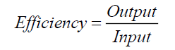
The most basic way to measure efficiency is by computing a ratio between a unit of output and a unit of input:
However, the above circumstance is very rare as most organizations and firms operate with many inputs and outputs. Thus, this efficiency measure can be explained as follows:
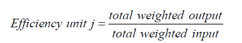
Which can be further explained as:
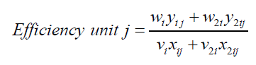
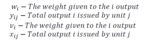
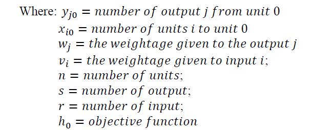
Where,
CCR Model
The CCR model is pioneered by Chames et al. (1978) and it is the most basic model in the DEA. The efficiency of the decision-making unit is defined as the rate of total weighted output  divided by the total weighted input ,
  it is known as the CCR model:
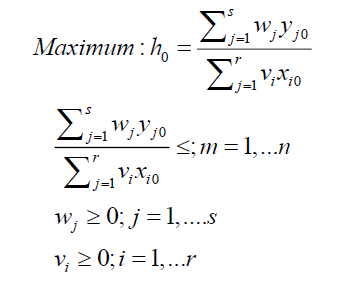
The W and V values are the weightages for each output and an unknown input and this means that each unit is free to determine its weightage set factors which will make the set as effective as possible within its constraints. This efficiency will eliminate the difficult step when determining appropriate weighting factor for each input and output. These units are said to be relatively efficient if the final decision  is equal to one, but the weighting combination is not necessarily unique. If the final result of
  values is less than one, then the unit is said to be less efficient and there is no weighting combination that may allow it to be efficient.
BCC Model
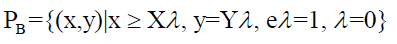
The BCC model has been introduced for the first time by Banker et al. (1984) and used to measure technical competence. The efficiency score obtained from this model will give the score at least the same as the score obtained using the CCR model. The set of production for the BCC model is explained by the following equation:
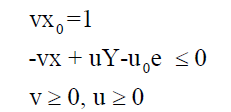
BCC model describes the morning efficiency of each DEA  by completing the following linear program:
Min  subject to:

Which, the BCC dual program can be described as:

Subject to:
Generally each unit uses a set of resources called an input set to produce a set of outputs called an input set. The function of each unit is to change the input set to the output set and the relative efficiency is measured based on the efficiency of the conversion of the total output produced for each input unit (Boussofiane et al., 1991). For a clear picture, assume a sector has P unit, X using as input and Y as output. Unit k0 is said to be efficient if there is no other unit or other unit combination that produces at least one output greater than unit without reducing the other output or at least one other input. Unit can also be said to be efficient if no other units or other unit combinations produce the same output level but use one of less inputs without using more than k0 units for at least other inputs (Charnes et al., 1978).
For this study, the output-oriented DEA method is used to determine the efficiency of the sub-sectors obtained. In contrast, for output-oriented DEA, linear programming models are used to determine the potential output that can be produced at the “best boundary practice” when the input factor is in constant value. This approach is more analogous in determining the output potential of the specified input set and the capacity as a ratio to the actual output potential. In other words, the output-oriented DEA approach is generally more appropriate in assessing the use of capacity to produce performance indicators.
As mentioned, DEA measurements should involve all relevant factors that are classified as input or output into the model. In this study, the inputs and outputs chosen must also be at a balanced level. This is because no single factor is given priority over other factors. Additionally, DEA is used to measure relative efficiency with the best practice performance compared to other techniques that are based only on average observations or some previous performances that have been done. Apart from identifying inefficient units, the DEA measurement results are valuable as they can be used to determine the steps that need to be followed to improve the efficiency of the incomplete units (El-Mahgary & Ladelma, 1995).
Results and Discussion
The performance indicators for the processing industry are determined by reference to technical efficiency and scale as shown in Table 1. The CCR model is used to determine the relative efficiency of fixed returns to scale (FRS) technology. Because FRS technology is a neutral scale, it can be assumed that all decision-making units (DMU) operate on an optimum scale. In another perspective, the BCC model is used to determine the efficiency under change returns to scale (CRS) technology and to allow the possibility that an inherent inefficiency may occur due to the value of DMU which deviates from their respective operational scale, as well as due to the technical inefficiency. In the DMU concept, the boundary production function is used to determine the best practices among all DMU data samples. As the capability for each DMU to exceed the boundary limit varies, so it is realistic that the change returns to scale (CRS) technology is used to determine the efficiency of an industry. The value of the competency index corresponding to one implies that the industry is at the best practice boundary while the values below one implies that the industry is under borders or technically inefficient.
| Table 1: The Analysis Of Model Ccr And Bcc | ||
| Year | Model CCR (FRS) | Model BCC (CRS) |
|---|---|---|
| 1993 | 0.610 | 0.678 |
| 1994 | 0.857 | 0.932 |
| 1995 | 0.812 | 0.846 |
| 1996 | 0.928 | 0.947 |
| 1997 | 0.900 | 0.927 |
| 1998 | 0.865 | 0.900 |
| 1999 | 0.916 | 0.976 |
| 2000 | 0.931 | 0.937 |
| 2001 | 0.860 | 0.894 |
| 2002 | 0.934 | 0.936 |
| 2003 | 0.910 | 0.933 |
| Average | 0.865 | 0.900 |
Based on the findings obtained, most industries recorded a high overall efficiency rating under the BCC model. If the DEA provides a negative value of technological change, it does not mean that an industry has a low technical efficiency. This is because a fully competent industry is unable to increase the amount of output at fixed-given inputs on a regular basis; however it is able to set the boundaries forward by adapting new technologies. At the same time, positive technology changes can be achieved by enhancing technology management in every production process, for example: machinery usage, skilled labour, effective automation systems, and product development, as well as products innovation that meet targeted standards.
| Table 2: The Efficiency Of Ccr And Bcc Models In 1993 | ||
| Sub-sectors | Model CCR (FRS) | Model BCC (CRS) |
|---|---|---|
| Coconut | 0.694 | 1.000 |
| Palm Oil | 1.000 | 1.000 |
| Cocoa | 0.478 | 0.496 |
| Coffee | 0.339 | 0.360 |
| Rubber | 0.171 | 0.301 |
| Rice | 0.589 | 0.591 |
| Wheat | 1.000 | 1.000 |
| Average | 0.610 | 0.678 |
With reference to Table 2, the average technical efficiency score yields 1.00 under the CCR model and also 1.00 under BCC model to two sub-sectors namely palm oil and wheat; while other sectors show higher BCC index values than CCR. In the years of 2000, 2001, and 2002, the efficiency index for the rubber sub-sector had decreased the index for both models at around 0.50 to 0.70 (not shown here) while the other sub-sectors did not show any changes. Overall, performance scores based on the CCR model recorded lower values than the BCC efficiency values and logically, this condition may have been due to the BCC distance function which is closer to the production boundary than CCR. This resulted into a higher BCC index since the ratio of the distance from the input line is closer to the boundary and thus increasing the efficiency index value. A basic picture of distance function can be viewed at Figure 1.

Figure 1.Distance Function Model For Bcc And Ccr.
Based on Figure 1, there are four points shown namely the points (A, B, C & D). All of these points are used to estimate the boundary efficiency and level of capacity utilization under both assumptions of scale. The graphical boundary shown above indicates the full output capacity given to several input levels. Referring to CCR model; point C exists amid the boundary with other points being below the boundary (indicating weak capacity utilization). For BCC, the boundary is indicated by points A, C and D with only B situated below the boundary line (indicating weak capacity utilization). By conducting analysis, capacity utilization is determined by allocating the ratio between actual output to output boundary levels. By excluding point C, (having 100% capacity utilization under both assumptions model) determination of capacity utilization per point is low when assuming to CCR than BCC model. The output capacity shown by the BCC model is lower than the CCR output capacity. Hence, it may be assumed that CCR boundaries are more exposed to higher output capacity values compared to BCC boundaries. At the same time, the BCC boundary is more susceptible to higher capacity utilization compared to the CCR boundary.
Looking at the efficiency wise, the agricultural-based processing industry can be assumed to have optimum scale of optimum efficiency for most of the year except in 1993; while the highest average efficiency score was recorded in 2002 (Table 3) with almost all values were recorded with perfect score. Notwithstanding the rubber sector which has a significant decrease of 0.540 for CCR model and 0.549 for BCC model, the efficiency score scale assumes that there is a deviation from the operating scale but is still approaching to value of one over time.
| Table 3: The Efficiency Of Ccr And Bcc Models In 2002 | ||
| Sub-sectors | Model CCR (FRS) | Model BCC (CRS) |
|---|---|---|
| Coconut | 1.000 | 1.000 |
| Palm Oil | 1.000 | 1.000 |
| Cocoa | 1.000 | 1.000 |
| Coffee | 1.000 | 1.000 |
| Rubber | 0.540 | 0.549 |
| Rice | 1.000 | 1.000 |
| Wheat | 1.000 | 1.000 |
| Average | 0.934 | 0.936 |
Conclusion
With reference to the analysis carried out, it is found that BCC efficiency model is much higher than the CCR efficiency model in almost all efficiency indexes. This is because; it is relatively difficult to fully achieve an efficient industry (which is by increasing the amount of output at given inputs on a regular basis). However, this can be made possible by setting boundaries forward through adaptation of new technologies. The results from the model found that the sub-sector of rubber has recorded the lowest efficiency index during the entire study period with index as low as 0.171 for the CCR model and 0.301 for the BCC model in 1993. On the other hand, other sub-sectors such as coconut oil, palm oil and wheat industries, those industries did not experience any change in efficiency and remained at the value of one throughout the study period from 1993 to 2003.
It is practical to acknowledge that execution of the preceding two national agricultural policies since 1984 has permitted the agricultural sector to achieve a growth rate of efficiency for most of the commodities. The strategies taken under the agricultural policies (The First and Second NAP) qualified for a good merit due to the fact that these two policies had given the authorities a chance to develop new agricultural land to equip the formation of economic farm units. Well-organized agricultural practices have been adapted and land has been allocated to agricultural farmers for planting new crops. Institutional development of land was also put through in order to fix the issues of unproductive farm sizes, unproductive crops and shallow levels of productivity, while not neglecting the agricultural support services like research, extension, marketing, fiscal incentives and social and institutional development.
As stated earlier, it is highly expected that achievement of agricultural sustainability would bring about self-sufficiency in foods due to the lack of comparative advantage in producing many food commodities. With introduction of the Third National Agricultural Policy, it is shown that the Malaysian agriculture sector has been given a new rent of life in order to become an engine of economic growth.
It is indispensable that agriculture is the main economic thrust for Malaysian rural communities. At the same time, it is also substantial that during the Ninth Malaysian Plan period (2006-2010), the agriculture sector obtained a higher rate of growth than targeted and contributed towards economic growth and export earnings, in which there was an improved involvement of the private sector in large-scale commercial food production and agro-based industry. In addition, the development of the agriculture sector has been intensified to serve as the third engine of growth during the same period. In fact, the contribution of Malaysian agricultural sector to the national economy is remarkable particularly in creating employment, alleviating rural poverty and reducing net export deficit. It is expected that the Ministry of Agriculture is going to adopt more target specific policies and strategies to further accelerate the transformation of the agriculture sector into a modern, dynamic and competitive sector pertinent to agro-based processing activities and agricultural entrepreneur development.
References
- Ahmad, F.P. & Rohana, A.R. (2006). Key sectors in the Malaysia economy to accelerate economic growth. Universiti Putra Malaysia Press, 70-89.
- Banker, R.D., Charnes, A., & Cooper, W.W. (1984). Some models for estimating technical and scale inefficiencies in data envelopment analysis.Management Science,30(9), 1078-1092.
- Beasley, J.E. (1990). Comparing university departments.Omega,18(2), 171-183.
- Boussofiane, A., Dyson, R.G., & Thanassoulis, E. (1991). Applied data envelopment analysis.European Journal of Operational Research,52(1), 1-15.
- Chames, A., Cooper, W.W., & Rhodes, E. (1978). Measuring the efficiency of decision making units.European Journal of Operational Research,2(6), 429-444.
- Cho, G. (2011).The Malaysian economy: Spatial perspectives. Routledge.
- Courtenay, P.P. (1987). Malaysia's National Agricultural Policy: Experimental systems in the padi sector.Land Use Policy,4(3), 294-304.
- El-Mahgary, S., & Lahdelma, R. (1995). Data envelopment analysis: visualizing the results.European Journal of Operational Research,83(3), 700-710.
- Indrani, T., Siwar, C., Hossain, M.A., & Vijian, P. (2001). Situation of agriculture in Malaysia-A cause for concern.Education and Research Association for Consumers Malaysia.
- Mad Nasir, S., Zainalabidin, M., Md Ariff, H., Zulkornain, Y., & Alias, R. (2012). The empirical evaluation of productivity growth and efficiency of LSEs in the Malaysian food processing industry.International Food Research Journal,19(1).
- Mahfoor, H.H., Mad Nasir, S., & Ismail, A.L. (2001). Challenges for agribusiness: A case for Malaysia. InInternational Symposium on Agribusiness Management towards Strengthening Agricultural Development and Trade, Chiang Mai University.
- Mat Nasir, S. & Ghazali, M.M. (2007). Agriculture and Agribusiness in Malaysia: Performance and strategies for growth, Universiti Putra Malaysia Press, 28-54.
- Matahir, H., & Tuyon, J. (2013). The dynamic synergies between agriculture output and economic growth in Malaysia.International Journal of Economics and Finance,5(4), 56-71.
- Ministry of Agriculture and Agro-Based (n.d.). Overview of the Agriculture Sector in Malaysia. Retrieved from http://go2travelmalaysia.com/
- Murad, W., Mustapha, N.H.N., & Siwar, C. (2008). Review of Malaysian agricultural policies with regards to sustainability.
- Murad, W., Mustapha, N.H.M., & Siwar, C. (2009). Review of Malaysian agricultural policies with regards to sustainability.American Journal of Environmental Sciences,5(1), 728-734.
- Muzafar, S.H. (2006). Engine growth in the states of Malaysia: Has the role of agriculture sector diminished? Universiti Putra Malaysia Press, 90-103.
- Norman, M., & Stoker, B. (1991).Data envelopment analysis: The assessment of performance. John Wiley & Sons, Inc..
- Okposin, S.B., Halim, A., Hamid, A., & Hway, B.O. (1999).The changing phases of Malaysian economy. Pelanduk.
- Rasiah, R., & Shari, I. (2001). Market, government and Malaysia's new economic policy.Cambridge Journal of Economics,25(1), 57-78.
- Shapira, P., Youtie, J., Yogeesvaran, K., & Jaafar, Z. (2006). Knowledge economy measurement: Methods, results and insights from the Malaysian knowledge content study.Research Policy,35(10), 1522-1537.
- Shobri, N.I.B. M., Sakip, S.R.M., & Omar, S.S. (2016). Malaysian standards crop commodities in agricultural for sustainable living.Procedia-Social and Behavioral Sciences,222, 485-492.
- Wong, L.C. (2007). Development of Malaysia’s agricultural sector: Agriculture as an engine of growth. InConference on the Malaysian Economy: Development and Challenges.
- Yusof, M.S., Alias, R. & Amin, M.A. (2006). The role of the agricultural sector in the malaysian economy. Universiti Putra Malaysia Press, 1-27.