Keywords

Financial Analysis, Capital Structure, Capital Management, Financial Stability, Agriculture

Introduction

One of the most controversial issues of financial management is the problem of finding the optimal capital structure. The practical significance of this definition is very significant since it is essentially a direct continuation of the issue of the cost of capital and a source of continuous development of the company. It also plays a key role in shaping the financial stability of an economic entity.

Agriculture is a key component of the economy of any country. The issues of the financial state for this industry are quite acute since the specifics of doing business have a high level of risk of loss of financial stability.

According to the Federal State Statistics Service (Agriculture in Russia (statistical digest), 2019), the number of organizations operating in crop and livestock production, hunting, and providing related services has decreased by 80% since 2000. All this creates a negative trend to reduce competition in the agricultural production market, which leads to additional risks. However, even in these conditions, the number of unprofitable enterprises remains at a very high level (26.2%) as of 2018 (Table 1 & Figure 1).

Table 1 Financial Results of Organizations Engaged in Crop and Livestock Production, Hunting And Providing Related Services
	2000	2014	2018
Number of organizations for the reporting period, thousand including:	27.7	5.9	5.2
profitable organizations	13.7	4.3	3.8
unprofitable organizations	14	1.6	1.4
Share of profitable organizations in the total number of organizations, percent	49.3	73.6	73.8
Share of unprofitable organizations in the total number of organizations, percent	50.7	26.4	26.2
Amount of profit, million rubles	36878	264044	302606
Amount of loss, million rubles	20748	82973	96435

Figure 2 Profit and losses incurred by enterprises operating in crop and livestock farming & hunting and the provision of related services in these industries, in million Russian Ruble

In many ways, the Modigliani-Miller theorem became the starting point of the scientific discussion on the optimal ratio of own equity and borrowed capital. In its first generation (Modigliani, & Miller, 1958), it has been proved that the market value of an enterprise does not depend on the structure of its capital and is determined by the capitalization rate of expected income in the enterprises of the same type. One of the main assumptions of this theorem is the absence of taxes on corporate profits and on personal income, the absence of transaction costs, an ideal capital market, the absence of information asymmetry, and others.

The next stage in the development of the theory was the accounting of corporate income tax (Modigliani & Miller, 1963). Based on the fact that the company has a tax shield (in case of debt financing, the interest on the loan reduces the tax base for income tax), the value of the company with debt financing is higher than of the company with its own financing.

The theory was further developed in 1977 in the works of M. Miller and other theorists, who developed compromise theories and theories of the hierarchy of finance in relation to the structure of capital.

The compromise models developed by Kraus, Litzenberger, De Angelo, Kim, Bradley (Braley & Myers, 2008; De Angelo & Masulis, 1980) and other authors use factors that take into account the costs associated with financial difficulties, as well as agency costs.

They came to the conclusion that as the share of borrowed capital increases, it becomes more difficult and more expensive for a company to attract new loans. Thus, it is particularly important to choose a capital structure that has the maximum positive effect when taking into account the factors affecting it.

Financial hierarchy theories are based on empirical research on the financial structure of enterprises operating in different countries. The fundamental work in this area was the work by Gordon Donaldson (Donaldson, 1961). He analyzed the actual practices of forming the capital structure of American companies, which are relevant for Russian enterprises:

• Companies prefer to use internal reserves (retained earnings, depreciation and amortization) in financing, rather than to attract them from outside;

• The dividend policy is organized to make the dividend payments constant in short term, and after the dividend payout, the company would have a sufficient amount of retained earnings to finance its activities. With an increase in dividend payout, there is a possibility that it would be difficult to maintain them at this level, and with a decrease in dividends, the investment attractiveness of shares decreases;

• If there is a surplus of capital that the company is not able to invest in the close future, it is more likely to invest it in fluid market instruments but it is less likely to return some of the borrowed capital, or, even less likely, to raise the dividend, or buy back some of its own shares;

• If there is a lack of own funds to finance investment projects, the company will initially sell fluid market instruments, and only then will it attract external financing, e., first it will try to attract a loan, then it will issue loan stocks, and only last of all it will issue ordinary shares.

Donaldson identified a hierarchy of management preferences in the formation of the financing structure that influenced the arguments of compromise theories. However, the empirical approach is also typical of high subjectivity, and therefore its conclusions are basically introductory.

The models mentioned above have a high theoretical potential but in a practical sense, having so many assumptions, they are difficult to apply. Thus, it is necessary to assess the capital structure systematically, evaluating all its components in symbiosis.

To implement this task, the study proposes a Model of the Financial Structure (MFS) that allows to determine a balance between aggregated groups of assets by fluidity and groups of liabilities by the degree of urgency of their payment in the course of current activities, to reduce the financial costs associated with attracting sources of financing, to increase their efficiency, and reduce to the risk of loss of solvency.

Materials and Methods

This study used general scientific methods: system analysis, methods of dynamic, factorial, and comparative analysis, modeling, as well as specific tools for the formation of balanced indicator systems and aggregated indicators. The use of modern mathematical, statistical and other modern methods ensured a high level of reliability of the conducted research, as well as the most complete study of the problems.

When forming the model, the study considered the relation between the resources and funding sources of the enterprise (presented below in Scheme 1), and the conditions of equilibrium between the aggregated groups of assets and liabilities necessary to maintain the financial stability of the organization in market conditions.

The main tools of the MFS model are: financial leverage that describes the quality of the structure of sources of funding; the price of attracting financing sources that describes the level of risk associated with the selected financing structure; the effect of financial leverage that allows determining the feasibility of using borrowed capital.

Section 1 "The Price of Own Funds"

To determine the price of own sources of funding, it is proposed to divide them into two groups: starting own equity (SOE_start )and own equity accumulated during economic activity within the period of operation (SOE_acc):

SOE = SOE_start+SOE_acc

Own accumulated capital includes Reserve Capital (RC) formed from net profit, Additional Capital (AC) and retained or Reinvested Earnings (RE):

SOE_acc= RC+AC+RE

The retained earnings of the period is the difference between the net profit and the dividends paid. It is the main component of the increase in the wealth of the owners and contributes to the increase in the capitalization of the company. Its size depends on the efficiency of the company's activities and the economic policy including the dividend policy. Non-payout of dividends, even if the financial results are good, automatically affects the interest of investors in its securities and negatively affects their value. However, a high level of dividends may become an important factor in the degradation of the enterprise and jeopardize the renewal of its funds. A balanced approach to paying dividends and building economic potential leads to an increase in investment attractiveness, the market value of the enterprise, and the income of the owners.

When assessing the cost of equity, it is proposed to take into account interest accrued for borrowing in addition to dividends, penalties, etc., which arise as a result of inefficient management. The amount of interest payable on borrowed capital reduces the profit. It depends not only on the average interest rate of the credit institution but also on the work of the company's financial management. Taking these factors into account allows determining the level of risk associated with each component of the exchange system and set a minimum threshold for the profitability of own equity.

The cost of the initial capital (ordinary and preferred shares) is determined on the basis of the amount of dividends paid by the company to the share owners. It is necessary to take into account the size of preferred and ordinary shares per year.

Cdiv_t = DV_t : L_t

Preferred shares are actually the borrowed capital. The payout of dividends is carried out at any financial results, even if there are losses. The price of the preferred shares is known in advance(C_prsh ).

Dividends attributable to ordinary shares are paid out of the net profit allocated for the dividends payout minus dividends on preferred shares, as decided by the shareholders' meeting.

CiCt = (Cprs×dprs+Cors×dors):L,

The cost of the initial capital in the t-th period is as follows:

Where Cprs is the cost of preferred shares;

dprs is share of preferred shares;

Cors is the cost of ordinary shares;

dors is the share of outstanding ordinary shares.

The amount of equity capital is negatively affected by penalties (P) that have arisen as a result of inefficient management and late payment of obligations to counterparties: they reduce the amount of net profit and the amount of own equity accumulated as a result of economic activities. The amount of penalties per ruble of own equity accumulated as a result of economic activity is determined by the formula:

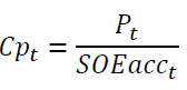
To identify trends in the price of start-up capital, taking into account the possible spread of its values, the study uses weighted averages.

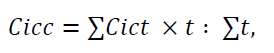
Cict – the amount of dividends on the shares of the enterprise authorized capital attributable to one ruble of the authorized capital in the t-th period of time, t=1, T

The value of the indicatorC_p for several previous periods allows to determine the level of owners' losses as a result of inefficient management and to use it when drawing up forecast plans (Cpcc ):

where

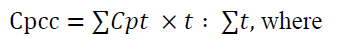
Cpent - the amount of penalties per one ruble of own equity in the t-th period of time, t=1, T

Increasing the pace of economic development is impossible without the use of borrowed capital. The greater the need is, the greater is the interest to be paid for their use. The amount of these financial costs depends on the level of financial stability of the enterprise: the worse the financial condition of the enterprise is, the higher is the interest rate of the economic feasibility of investments, the quality of financial managements in the formation of a portfolio of borrowed capital for several previous periods. Therefore, when predicting the level of financial stability, it is necessary to monitor the dynamics of the average amount of interest payable (Ipay) per ruble of own equity accumulated as a result of economic activity (SOEacc).

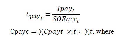
Cpayt – the value of the coefficient Cpay in the t-period, t=1, T

The coefficients Cpc,Cicc,Cpayc carry an important economic meaning: they allow determining the lower threshold of the effectiveness of own equity (Teoe ):

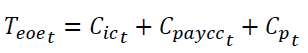
The return on own equity threshold reflects the minimum level of own equity efficiency. It should be used to determine the level of the margin of safety of own equity in the t-th period.

The margin of safety of own equity allows taking into account the return on own equity, for example, on Earnings Before Taxes and Interest (EBIT):

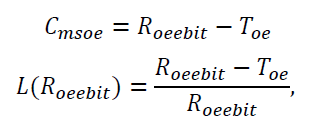
- margin of safety of own equity;

 

R_oeebit- return on own equity on earnings before taxes and interest (EBIT);

The higher the value of the indicator L(R_oeebit)is the more effective is the management of funding sources, which affects the level of financial stability.

The value (T_oe ) is necessary to predict the minimum return on own equity for the next (t+1) period for the normal and uninterrupted operation of the enterprise.

As a result of changes in the operating environment, the possible adjustments for each component should be considered.

The lower threshold of profitability of own funds is determined by the formula:

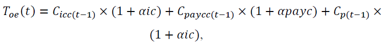
where αic, αpay, and αic are the adjustment coefficients for each component, respectively.

The value T_oe (t) shows how much of the own equity can be withdrawn in the course of the activity as a result of the decisions made on profit distribution, on the dividend policy, and on the use of borrowed capital.

The price of own sources should be adjusted for the inflationary component:

– the cost of own equity; Jnfl – the level of inflation in relative terms; T_oe - the threshold of return on own equity; T_pr - the minimum threshold of profitability for business owners.

The calculation of the price of own equity using this formula allows taking into account inflationary risks, the margin of owners, and more accurately determine the price of common sources of funding necessary to support the activities of the enterprise (Petrovskaya, Larionova, Zaitseva, Bondarchuk, Grigorieva, 2016).

Section 2 "The Cost of Borrowed Capital"

In addition to own equity, borrowed capital play an important role in the financing structure of the enterprise. When determining the cost of borrowed capital, it is necessary to take into account the structure and role of each of its components in financial resources.

The model based on the results of the analysis for previous periods takes into account the average share of each component and the fee for attracting. The cost of borrowed capital in the t–th period is determined by the formula:

– cost of borrowed capital in the t-th period;

Ipaylbft – interest payable on long-term borrowed capital in the t-th period,

Ipaysbft – interest payable on short-term borrowed capital in the t-th period,

CSsapt-the cost of servicing accounts payable in the t-th period;

lbft – long-term borrowed capital in the t-th period;

stbft - short-term loans and borrowings in the t-th period;

apt – accounts payable in the t-th period.

Determining the cost of borrowed capital according to the formula allows to identify the influence of the listed factors in each t-th period on the cost of the borrowed capital (Cbc) and to determine the trends of their changes.

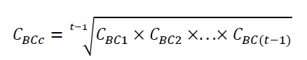
When predicting the minimum return on borrowed capital for the next (t+1) period, it is proposed to use the geometric mean of the cost of borrowed capital:

If we take into account the price of borrowed capital for the t-th period and possible changes in the influencing factors for each component of the cost, then the cost of borrowed capital for the next (t+1) period should be calculated using the formula:

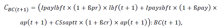
where ßpr, ßpay, and ßcr are the correction factors.

This approach allows to take into account the quality of debt management over the past periods, make appropriate adjustments, and, consequently, reduce the likelihood of errors in making forecasts, increase the reliability of projected calculations, and more realistically approach the optimization of borrowing costs, taking into account changes in the trends of influencing factors.

Section 3 "Weighted Average Cost of Capital'

Accounting for the cost of own equity and debt capital allows to calculate a key indicator that characterizes the price of capital of an enterprise in each t-th period using the Weighted Average Cost of Capital (WACC):

– the share of own equity in the structure of sources of financing; - the price of own equity; Citt - the estimated income tax rate, determined on the basis of the company's financial statements; - the share of borrowed capital in the structure of sources of funding; C_BCT- the adjusted cost of borrowed capital in the t-th period with the annual interest rate on this type of loan and the amount of interest accrual during the year.

The WACCt value characterizes the minimum level of return on the invested capital of the enterprise, the threshold of its break-even in the t-th period.

The real rate of return in the t-th period (Rrat) and for the analyzed period of time is determined by the formulas:

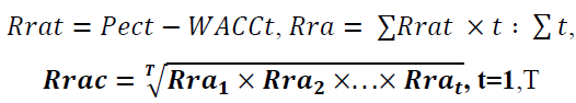
Obviously, the increase in the non-negative value of Rrat shows the success of doing business. Vice versa, the decline in the dynamics of the Rrat indicates an increase in the risk associated with the formation of the financing structure of resources, as well as their effective use.

The average value of the Rrat allows setting minimum targets for business performance in the future. Obviously, the return on invested capital and the rate of return should satisfy the following relations:

The value of the cost of borrowed capital serves as a basis for assessing the quality of the structure of funding sources, the efficiency of own equity due to the use of borrowed capital despite their payment in each t-period. The calculation of the level of financial leverage is as follows:

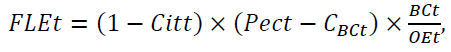
– the effect of financial leverage, %; Citt – the estimated income tax rate in relative terms; Pect – economic profitability,%; C_BC- the cost of borrowed capital,%; BCt – borrowed capital; OEt-equity, t - t-th period.

If the FLEt value is positive, then the chosen structure of financing sources for the t-th period, despite the payment of borrowed capital, would increase the efficiency of own equity, and, consequently, would favorably affect the level of financial stability. A negative FLEt value increases the level of financial stability risk. This is a signal to identify the reasons for the deterioration of the structure of funding sources. In this case, it is advised to use a factor analysis method that allows to determine the impact of changes in each influencing factor of the model on the reduction in the effectiveness of own equity.

Results

There are several options for choosing the structure of funding sources based on the possibility of using each component to a sufficient extent and the use fee. Therefore, the task of managers is to choose the most acceptable option from a set of alternative options (B = (B_l), l=1,L)..

The formalized model of the financial structure of funding sources in the t-th time period can be presented as follows:

Cbct=(1+ ß)×Cbcc?,C?_BCc=√(t-1&C_BC1×C_BC2×...×C_(BC(t-1)) )

Cbct=(Ipaylbfct×lbft+Ipaysbf?t×stbft+CSapt×apt): BCt,

C_oet=(1+Inflt)×(1+T_eoet )×(1+?Int?_oet )-1,

T_eoe (t)=C_ic(t-1) ×(1+αic)+C_(paycc(t-1))×(1+αpayc)+C_(p(t-1))×(1+αic)

FLEt=(1-Cittc)×(Pect-C_BCt )×BCt/OEt>0

Pect>WACCt; . Rrat≥ Rra(t-1)>0

Discussion

The problem of assessing and predicting the optimal structure of own equity and debt capital is an important aspect of studying the economics of enterprises in various industries. Research in this area is of particular importance for activities that are related to a high risk of loss of financial stability, for example, agricultural production.

Based on the works of various authors (13, 15, 19, 20, 21), this study reveals the following specific features of the activities of agricultural enterprises, which carry additional risks of loss of financial stability:

High exposure to natural-climatic and epidemiological risks (risk of loss of crops or livestock);

Seasonality of production (additional expenses, uneven flow of revenues);

Impossibility of obtaining several harvests per year in the climatic conditions of the Russian Federation (restriction of financial income);

Long production process (the need for planning and forecasting);

High dependence on the market conditions of agricultural products (the complexity of forecasting the income received);

The need for additional management qualifications in the field of biology, agronomy, animal science, veterinary medicine, etc. (complexity of personnel selection, additional training costs);

The above-mentioned risk factors require management to make adequate and timely decisions in the field of the financial condition of an economic entity. In turn, it makes it particularly important to develop a comprehensive system for assessing the cost of capital and the optimality of its structure.

Many researchers have contributed to the development of scientific knowledge in this field. They are Braley & Myers (2008); Fischer, Heinkel & Zechner (1989); Frank & Goyal (2009); Miglo (2016); Porras (2011); Khudyakova & Shmidt (2017); Petrovskaya, Larionova, Zaitseva, Bondarchuk, Grigorieva & Vasilieva (2016); Vasilieva, Shaporova, Tsvettsykh

The basis of the system is laid down by the theories and models proposed in the last century by Modigliani, Miller, De Angelo, Donaldson, Fischer, Altman, and other scientists. Thus, this issue reaches a qualitatively new level of research. However, all of these theories and models have a large number of assumptions which significantly complicates their practical application.

Modern works form a fairly high-quality tool for assessing the cost of capital and the optimality of its structure. It is worth highlighting the work of Vasilieva, et al., that optimizes and applies the capabilities and achievements of Edward Altman for agro-industrial enterprises.

An important point in the development of the assessment system was the creation of a basic approach based on integrated indicators of financial condition, which in particular are presented in the works of Khudyakova, Schmidt, Sekacheva, Skaryupina, Polinkevich and others. This approach provides high practical availability of scientific results.

The proposed systems for assessing the level of risk associated with the optimal capital structure factor should also be highlighted. This approach is applied in the works of Petrovskaya and others and allows to get a better assessment in the context of possible risks of loss of solvency.

It should be noted that the variety of approaches of different authors to optimizing the capital structure, on the one hand, gives users a lot of opportunities for evaluation and decision-making, but, on the other, significantly complicates the process of using the appropriate tools. In this regard, the task of forming an up-to-date universal method of assessment and forecasting applicable to enterprises in various sectors of the economy is of great importance.

Based on the optimal range of indicators, the study formed a model of the financial structure. It became the basis for a multi-factor assessment of the cost of own equity and borrowed capital, the calculation of the threshold for the effectiveness of equity and its margin of safety, the weighted average cost of capital and the real rate of return of the enterprise. All this concluded the maximum analytical potential, which significantly simplifies the process of making a management decision in a simple form.

Conclusion

The presented model allows to assess the actual level of the capital structure and maintain the achieved optimal level of financial stability in the long term, serves as the basis for financial control of the structure of funding sources in case of changes in the operating environment and the level of business activity.

The inclusion in the cost calculation of the maximum number of factors that affect the cost of capital, in particular, reflecting inflationary risks, penalties, the turnover of the company's shares, the dynamics of interest payable, and so on, reveals the most complete picture based on the results of analyses.

In addition, the company management is given the opportunity to form target settings when predicting the company's future financial position. It simplifies the use of this tool and allows it to adapt to various conditions of the external and internal environment of the enterprise.

References

1. Braley, R., & Myers, S. (2008). Principles of corporate Finance, (2nd edition). Moscow, Olimp-Biznes.
2. De Angelo, H., & Masulis, R.W. (1980). Optimal capital structure under personal and corporate taxation. Journal of Financial Economics, 8, 3-29.
3. Donaldson, G. (1961). Corporate debt capacity: A study of corporate debt policy and the de-termination of corporate debt capacity. Boston: Division of Research, Harvard Graduate School of Business Administration.
4. Fischer, E. O., Heinkel, R., & Zechner, J. (1989). Dynamic capital structure choice: Theory and tests. Journal of Finance, 44(1), 19-40.
5. Frank, M.Z., & Goyal, V.K. (2009). Capital structure decisions: Which factors are reliably important? Journal of The Journal of Finance, 39, 1067-1089.
6. Khudyakova, T.A. & Shmidt, A.V. (2017). Developing integrated performance assessment and forecasting the level of financial and economic enterprise stability. SHS Web of Conferences. EDP Sciences, 35.
7. Miglo, A. (2016). Capital structure in the modern world. Publisher Palgrave Macmillan. DOI 10.1007/978-3-319-30713-8.
8. Modigliani, F., & Miller, M.H. (1963). Taxes and the cost of capital: A correction. American Economic Review, 53, 433–443, 89.
9. Modigliani, F., & Miller, M.H. (1958). The cost of capital, corporation financing and the theory of investment. American Economic Review, 48, 261–297.
10. Petrovskaya, M.V., Larionova, A.A., Zaitseva, N.A., Bondarchuk, N.V., & Grigorieva, E.M. (2016). Methodical approaches to determine the level of risk associated with the formation of the capital structure in conditions of unsteady economy. International Journal of Environmental & Science Education, 11(11), 4005-4014.
11. Petrovskaya, M.V., Zaitseva, N.A., Bondarchuk, N.V., Grigorieva, E.M., &Vasilieva, L.S. (2016). Scientific methodological basis of the risk management implementation for companies’ capital structure optimization. Mathematics Education, 11(7), 2571–2580.
12. Porras, E. (2011). The cost of capital publisher Palgrave Macmillan UK. DOI 10.1057/9780230297678.
13. Report on the Condition of Agricultural Insurance Market, Carried out with the State Support in the Russian Federation in 2016 (2017). Information Brochure. Moscow, Ministry of Agriculture, FSBU «FAGPSSAP».
14. Sekacheva, V.M., Skaryupina, M.B., & Polinkevich, A.B. (2016). Characteristics of financial stability evaluation of the agricultural organizations under the traditional analysis of financial condition. Mezhdunarodnyy nauchno-issledovatel'skiy zhurnal, 4-1(46), 92-95.
15. Scherbakov, V.V. (2011). The partnership of government and business in the insurance of agricultural risks: The challenges of the new time and prospects of development: Monograph. Moscow: Dashkov&Co.
16. Shaporova, Z.E., & Tsvettsykh, A.V. (2019). Methodological foundations of the reference normalized model of an agricultural holding financial stability. IOP Conference Series: Earth and Environmental Science. IOP Publishing, 315(2).
17. Shmidt, A., & Khudyakova, T. (2017). The development of the integrated indicators of assessing financial and economics sustainability of the enterprise. In: Proceedings of the 4th International multidisciplinary scientific conference on social sciences and arts SGEM, 981-988.
18. Vasilieva, N. (2019). Using a quantitative assessment of the bankruptcy probability model as a tool for assessing the financial condition of subjects of the agro-industrial complex. Indo American journal of pharmaceutical sciences, 6(3), 6907-6912.
19. Trubulin, A.I. (Ed.) (2018). Agrarian economy of Russia: problems and vectors of development: monograph [Agrarnaya ekonomika Rossii: problemy i vektory razvitiya: monografiya]. Krasnodar.
20. Petrovskaya, M.V., & Sukhanov, I.V. (2016). Formation of a balanced model of financial stability of agricultural enterprises [Formirovanie sbalansirovannoy modeli finansovoy ustoychivosti predpriyatiy APK]. Moscow: RUDN.
21. Agriculture in Russia (statistical digest) [Sel'skoe khozyaystvo v Rossii (statisticheskiy sbornik)] (2019). Federal State Statistics Service. Moscow.