Keywords

Monetary Policy, Credit Supply, Cash Reserve Ratio.

Introduction

Monetary policy is one of the most important macroeconomic stabilization tools for regulating or controlling the amount, cost, availability, and flow of money and credit in the economy. It is a deliberate measure taken by the monetary policy authority (Central Bank) to influence the money supply and credit condition in order to achieve macroeconomic objectives such as price stability and economic growth (Adewunmi, 2019). Monetary policy, according to Pinshi (2020), is a tool used to influence the volume and direction of money in the economy. The conduct of monetary policy by central banks is recognized for ensuring that macroeconomic objectives are met. Central banks all across the world employ monetary policy instruments like the bank rate, open market operations, reserve requirements, and other selective credit control tools to achieve their macroeconomic aims. The setting of monetary variable targets is also the responsibility of central banks.

Monetary policy management can take the form of direct or indirect control, as well as mechanisms such as interest rates, credit ceilings, and sectoral credit allocation. Market-based economies frequently use indirect control devices. The link between money supply and the monetary base determines the ability of the monetary authority (CBN) to effect suitable changes in monetary policy instruments. The monetary authority employs the discount rate and reserve ratio to impact the money supply in the economy, and bank reserves are an important part of the monetary base. The credit ceiling in Nigeria is largely intended to allow for domestic credit expansion, and its monetary repercussions on the balance of payments correspond to the expected growth in total liquidity demand in the country. Under credit ceilings, for example, the apex bank found it increasingly impossible to achieve the specified monetary goals. Indirect monetary control approaches entail controlling the money stock by manipulating the source of the monetary base through the use of open market operations (OMO), reserve ratios, and interest rates (Li et al., 2021; Dakasku et al., 2020; Rivel & Yirong, 2020).

Despite gradual financial sector deregulation and the beginnings of the transition to market-based monetary management, Nigeria's ability to conduct efficient monetary policy has been impeded by a number of factors, the most notable of which is the absence of budgetary discipline until 1995. The efficiency of monetary policy in the post-structural adjustment programme (SAP) era has been hampered by a lack of instrument autonomy for the central bank, frequent policy changes, and widespread financial hardship also worth noting that, aside from the CBN's policy initiatives, the monetary authorities lack a true estimate of the amount of money in circulation in the economy. With the goal of improving performance, this study attempts to determine the effects of monetary policy on bank credit availability in Nigeria (Nyantakyi & Mouhamadou Sy, 2015).

Literature Review

Theoretical Framework

Monetary policy is a policy tool used by the federal government's apex bank to achieve the federal government's macroeconomic goals through the banking sector on a regular basis. These monetary policies have had an impact on the banking sector's activities and optimal performance over time. Monetary policy and bank operations are both founded on theoretical considerations.

Keynesian Theory

John Maynard Keynes is credited with developing the Keynesian theory of monetary policy in 1936. According to the theory, monetary policy should be based on interest rates rather than the money supply as a policy tool, and monetary policy should be second to fiscal policy. Monetarists think that monetary policy control is critical in macroeconomic management because of the close link between the monetary aggregate and economic activity. Commercial bank performance is influenced by a variety of factors, including macroeconomic, institutional, regulatory, and legal issues (Ekpung et al., 2015; Investopedia, 2015; Kareem et al., 2013). Because interest rate has an invisible influence on money supply, the Keynesian claimed that monetary policies should be focused on interest rate rather than money supply. Ekpung et al. (2015) went on to explain this with a model of the economic system's mechanism.

Where, OMO=Open Market Operation CBR=Commercial Bank Reserve MS=Money stock r=Interest Rate I=Investment GNP=Gross National Product

According to Ekpung et al. (2015), the open Market Operation (OMO) enhances the commercial banks reserve (R) and boosts the bank's reserves, assuming an economy in equilibrium and an open market purchase of government securities by the Central Bank of Nigeria (CBN) (2015). The bank then works to restore the desired ratio by issuing new loans or increasing bank credit in other ways. Additional demand deposits are created as a result of these new loans, increasing the money supply (MS). As the money supply expands, the general level of interest rate (r) decreases. Interest rates are falling, which has an effect on commercial bank performance and, as a result, increases investment due to the expected profit of businesspeople. Following rounds of GNP final demand spending increase by a multiple of the initial investment change due to the stimulated investment expenditure.

Monetarist Theory

Irvin Fisher is a significant proponent of the monetary theory (1911). A rise in the money supply, according to monetarists, enhances the actual percentage of money in relation to the desired proportion. The monetarist theory of money transmission mechanism can be expressed symbolically as follows:

This means that if the government conducts an open market operation (OMO), the money stock (MS) will rise, resulting in more expenditure and an increase in the gross national product, or GDP.

Empirical Literature

Morais et al. (2017) used bank data from 1980 to 2015 to investigate the impact of monetary policy on the supply of bank credit as a measure of banking sector performance in Mexico. The findings revealed that monetary policy shocks have an impact on credit supply in the banking industry. Low foreign monetary policy rates were also observed to have a greater influence on domestic borrowers.

Dhungana (2016) examined the impact of monetary policy initiatives such as the cash reserve ratio, open market operations, and the bank rate on bank lending in Nepal using data from 1996 to 2015. Panel data from 24 commercial banks was used in the study. Descriptive statistics, correlation analysis, and regression analysis were all used in the research. According to the data, open market operations and the cash reserve ratio had a negative influence on bank lending, whereas the bank rate had a favorable impact.

Akomolafe et al. (2015) examined the impacts of monetary policy on commercial bank performance in Nigeria using a micro-panel methodology. The interest rate and money supply were used to proxy monetary policy, while profit before tax was used to proxy commercial bank performance (PBT). Pooled regression, fixed effect regression, and random effect regression approaches were employed. Their studies revealed that bank earnings and monetary policy have a beneficial link. At 5%, however, the interest rate was determined to be minimal.

Employing data time series data 1981 to 2013, Apere & Karimo (2015) looked at the effects of monetary policy on the banking sector's performance. The authors used an unrestricted VAR (1) model method. Their research discovered that the direction of money supply reaction to a standard deviation structural monetary policy shock was not predictable. According to their findings, structural shocks in the monetary policy rate had a negative impact on money supply and banks' credit to the economy; nominal structural shocks had a positive impact on banks' credit to the economy; and money supply and banks' credit to the economy had a positive impact on banking sector reforms in the monetary policy rate.

Methodology

Model Specification

The Autoregressive Distributed Lag (ARDL) model is used in this investigation. Many writers, including Ewetan et al. (2015) have utilized this approach in a comparable study. The dependent variable in this model is believed to be a function of its own previous values as well as the current and past values of other variables (endogenous variables).

According to the structuralist paradigm, bank lending determines the deposit money supply. Inits most basic form, this may be written as:

We substitute deposit money supply (DMS) with banks total credit supply (BCS) and bank lending (BL) with interest rate (INR) since deposit money supply determines banks total credit supply to the economy and bank lending is driven by interest rate. As a result, when the monetary policy rate and the cash reserve ratio are included as extra monetary policy variables, equation (3.1) yields:

Where:

BCS = banks total credit supply MPR = monetary policy rate CRR = cash reserve ratio INR = interest rate

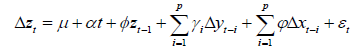
The bounds testing method entails estimating the autoregressive distributed lag model as follows:

Where:

is white noise error term

are parameters to be estimated

p=(1,2,... j) are lag lengths to be determined empirically using Akaike information selection criteria.

Data Sources

This study's data are time series data; hence they are considered secondary. The data was taken from the Statistical Bulletins of the Central Bank of Nigeria between 2009 and 2015. The data spans the years 1970 to 2015. However, this time frame is regarded adequate for the research, as it encompassed periods of various CBN monetary policies, including the move to market-based instruments from non-market-based instruments. Nigeria's financial sector was likewise hit by crises at this time.

Banking Sector Performance Index

This study used three indicators of banking sector performance to create a single index (or indicator) that proxied the performance of the whole banking sub-sector. Banks credit to the private sector, BCS (measure of allocation efficiency), banks deposit rate, BDR (measure of banks' level of attracting savings), and aggregate bank assets, (BA) covering aggregate bank asset are the indicators. The need for an index is justified by the fact that the measures are frequently highly correlated, but there is no general agreement on the best proxy. Furthermore, a single metric is insufficient to represent the entire banking sector's performance.

Using principal component analysis and a method similar to Ewetan et al. (2015), the three measures are converted into an index of banking sector performance as follows:

1. Given that BP'BI is a matrix made up of the following banking sector performance variables: [BCS, BDR, and BA], and that BP'BI is the 46 X 3 matrix of 46-year observations on the three performance indicators. The eigenvalues and eigenvectors of the BP'BI matrix produced are used to calculate the principal component.

2. The first eigenvector, belongs to the first principal component and corresponds to the highest eigenvalue. That is to say, In this case, the first principal component is the best measure since it better represents the changes in the dependent variable than any other linear combination of explanatory factors. As a result, just the first primary component's information is used to generate the index's loading and weights.

3. For BCS, BDR, and BA, the scoring coefficients sum of squares of the variables in the first main component are respectively. To get the loadings, we add the sum of the scoring coefficients as loading= .The weights for BA, BCS, and BDR used to generate the index are then calculated as follows:

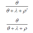
and

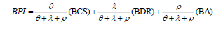
4. Therefore, the banking sector performance index (BPI) is constructed using the weights as:

Unit Root Test

In this study, the unit root of the variables would be examined using the Augmented Dickey-Fuller unit root test.

Augmented Dickey Fuller Unit Root Test

The Augmented Dickey–Fuller unit root test was used to establish the order of integration of the variables. However, Akaike's final Prediction Error (FPE) and Akaike's information criterion were used to empirically pick the lag order prior to the test. Table 1 summarizes the test outcomes. LDR, LR, and BDL are all stationary in their level forms. All of the order variables became stationary after the initial difference was taken. Because of the combination of I(0) and I(1) series, autoregressive models such as vector autoregressive and autoregressive distributed lag models are the best fit.

Table 1 Augmented Dickey – Fuller Unit Root Test Results
Variable	ADF – Statistic		Model	Lag order	Order of Integration
	Level	1st Difference
MPR	-1.648	-6.389*	Drift	1	I(1)
CRR	-3.104	-5.812*	Drift	1	I(1)
LDR	-4.080*	-	Drift	1	I(0)
INR	-1.520	-6.699*	Drift	1	I(1)
LR	-3.918*	-	Drift	1	I(0)
BPI	-2.332	-4.448*	Drift	1	I(1)
BCS	0.515	-4.361*	Drift	1	I(1)
BDL	-4.768*	-	Drift	1	I(0)

Cointegration

Co-integration is used to solve the problem of integrating short-run dynamics with longrun equilibrium. In essence, it demonstrates that co-integration may be used to make a linear combination of two non-stationary time series stationary. When two variables are co-integrated, it means they have a significant long-run relationship. In this scenario, a model that combines shortrun dynamics with long-run equilibrium is the most suited. Error Correction Models are the name given to such models (ECM). The presence of at least one co-integrating vector in the system is thus a sufficient condition for fitting an error correcting representation.

The bounds testing approach involves estimating the following equation.

Where:

= a column vector of dependent variables,x_t and y_t

is the first-difference operator.

The lag length is determined empirically using the model selection criteria of Akaike information.

The long-run multiplier matrix is:

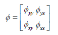
Because the matrix's diagonal elements are unbound, the chosen series can be either I(0) or I(1) (1). If yy then Y is I(1). If , on the other hand, Y is I(0). As a result, the test is also a unit root test.

The test hypothesis for the y_t equation is

Against the alternate

Results

Three banking sector performance indices are used in this study. Banks Credit to the Private Sector (BCS) is a metric that measures banks' allocation efficiency; Banks Deposit Rate (BDR) is a metric that measures banks' ability to attract savings; and Aggregate Banks Assets (BA) is a metric that measures total monetary assets. However, these indicators are highly correlated in most cases, and there is no consensus on which proxies are best for gauging banking sector performance. Furthermore, a single metric may not be sufficient to represent the entire banking sector's performance. This justifies the creation of an index that serves as a proxy for the overall banking sector's performance. As an overall indicator of the banking sector's performance, principal component analysis (PCA) is employed in a fashion similar to Ewetan et al. (2015) that appropriately addresses the concerns of multicollinearity and over-parameterization. We start with a correlation test of the banking sector performance variables (BCS, BDR, and BA), and the resulting correlation matrix is shown in Table 2:

The correlation matrix reveals that the variables are highly correlated. All of the correlation coefficients are more than 0.5. As a result, principal component analysis is utilized to combine the three performance proxies for the banking industry into a single principal component. Table 2 shows the findings of the principal component analysis. The first principal component explains 55.05 percent of the overall variation, the second component 28.93 percent of the entire variation, and the third component just 16.02 percent of the entire variation, according to the results. As a result, the best measure of banking sector performance is the first component, which contributes the most to the total variation of the variables. The first eigenvector, on the other hand, demonstrates that banks' assets and credit to the private sector are favorably associated with the first primary component, whereas banks' deposit rate is negatively correlated.

Table 2 Correlation Matrix
	BCS	BDR	BA
BCS	1.0000
BDR	-0.8410	1.0000
BA	0.7732	-0.8345	1.0000

Screeplot of The Eigenvalues of The Banking Sector Peformance

The standardized variance of the first primary component is 66.40 percent for bank assets and 58.36 percent for bank loans to the private sector, respectively. With a line across the y-axis at 1 and a heteroskedastic bootstrapping 95 percent confidence interval, the eigenvalues are also graphed. The plot is shown in Figure 1. The dark image shows the 95% confidence interval, the red line shows the Eigen values, and the three asterisk dots show the three components in the graph, respectively. The first component is the only one that is above the red horizontal line at 1, indicating that it is the most essential. This is in line with the results of the principal component analysis, which show that the first component should be preserved (Table 3). As a result, information about the first primary component is saved in order to calculate the index's loading and weights.

Table 3 Principal Component Analysis Result Used To Construct Financial Liberalization Index
Principal Component	Eigenvalues	Difference	Proportion	Cumulative %
1	1.65136	0.783324	0.5505	0.5505
2	0.868031	0.387418	0.2893	0.8398
3	0.480613	-	0.1602	1.0000
Eigenvectors
Variable	Comp1 (ρ1)	Comp2 (ρ2)		Comp3 (ρ3)
BA	0.6640	0.0902		0.7422
BCS	0.5836	0.5580		-0.5899
BDR	-0.4674	0.8249		0.3179

The scoring coefficients sum of squares of the variables in the first component for BA, BCS, and BDR, respectively, are 0.6640, 0.5836, and -0.4674. To calculate the loadings, multiply the sum of squares of the scoring coefficients by:

As a result, the weights for BA, BCS, and BDR utilized in creating the index are calculated as follows:

As a result, the banking sector performance index (BPI) is calculated as follows:

Trend Plots and Descriptive Statistics of the Variables

Trend graphs and descriptive statistics for the variables are discussed in this section. Plotting time series to acquire a sense of the series' trend is a popular activity. As a result, we plot the series, as shown below (Figures 3-5):

None of the series are mean reverting, and none of them are particularly volatile. The monetary policy rate fluctuated through time, with the highest rate recorded in the early 1990s, demonstrating that the monetary policy rate has changed through time. Although there are times when the trend is flat, such as in the mid-1990s, this indicates that the monetary policy rate remains steady. From the 1970s until the mid-2000s, when it trended upward until dropping abruptly in the mid-2010s, the bank performance index trended neither upward nor downward. This could indicate that the sector's performance was poor and remained thus in the years preceding 2010. The surge in the mid-2000s corresponds to the period of banking sector consolidation that began in 2005. As a result; one may argue that this is due to the period's consolidation program. Furthermore, the significant reduction in mid-2010 coincided with periods of weak banking sector performance, as indicated by post-consolidation crises in which institutions such as Bank PHB and others failed.

In addition, the descriptive statistics in Tables 4 a & b revealed that the mean values for MPR, CRR, LDR, LR, and BPI were 10.96739, 8.353868, 65.86966, 49.63429, and 2427017, respectively. As demonstrated by minimal standard deviation values, MPR, CRR, LDR, LR, and INR values in the data set cantered about their respective mean values (near to the mean value). However, as indicated by their exceptionally high standard deviation values, which are much larger than their mean values, the BPI, BCS, and BDL values are further from their respective mean values. All of the variables' minimum values are less than their respective mean values, with the exception of BPI, which is less than the mean value.

Table 4a Mean, Standard Deviation Maximum Values And Minimum Values
Variables	Mean	Standard Deviation	Minimum value	Maximum value
MPR	10.96739	5.206195	3.5	26
CRR	8.353868	6.434476	1	32
LDR	65.86966	12.03852	37.965	85.66147
INR	15.03545	6.273011	6	29.8
LR	49.63429	13.11123	29.1	94.5
BPI	2427017	4903585	1212.635	1.74
BCS	3179.427	5048.622	8.57005	18674.15
BDL	385806.6	982982.8	6.4	4132967

Table 4b Skewness And Kurtosis
Variables	Pr(Skewness)	Pr(Kurtosis)	Joint adjusted chi2(2)	joint p-value
MPR	0.1680	0.7845	2.09	0.3518
CRR	0.0001	0.0025	18.76	0.0001
LDR	0.1685	0.6793	2.19	0.3350
INR	0.7359	0.1914	1.92	0.3824
LR	0.0135	0.0562	8.41	0.0149
BPI	0.0000	0.0044	21.83	0.0000
BCS	0.0000	0.0143	17.96	0.0001
BDL	0.0000	0.0000	34.84	0.0000

The symmetry of a data set's distribution is referred to as skewness. Positive skewness coefficients indicate that the variables' distributions are completely symmetrical and right skewed. To put it another way, the scores of the individual factors were grouped to the left, with a right-hand tail. The peak of a distribution, on the other hand, is referred to as kurtosis. The Kurtosis coefficients are also comparable in terms of signs (all of the coefficients are positive), confirming peak. The skewness coefficients are all near to zero, with the exception of INR (0). With the exception of INR, this means that none of the variables deviates from the normal distribution. With the exception of LDR, MPR, and INR, which are all close to 0 and do not exceed it, all of the variables have a Kurtosis of less than 3 and are close to 0.CRR, LR, BPI, BCS, and BDL all have significant probability values at the 5% level, indicating that the hypothesis that these variables are normally distributed is rejected. However, at the 5% level of significance, the probability values of MPR, LDR, and INR are insignificant, indicating that the variables are normally distributed.

Monetary Policy and Banks’ Credit Supply

To determine if there is a level impact (cointegration) among the variables in the model, we use the Pesaran, Shin, and Smith (2001) Bounds test to estimate equation (3.3). Table 5 summarizes the results of the test. The F-value is 4.54, and the 95 percent upper and lower bounds are 3.23 and 4.35, respectively. We reject the null hypothesis of no level form relationship since the F-value is bigger than the upper limit. The fact that the t-statistics value is less than the 95 percent lower bound crucial value backs this up.

Table 5 Bounds Test Results For Level Form Relationship (Level Effect) Of The Variables
Critical Values (0.1-0.01), F-statistic, Case 3
90%		95%		97.5%		99%
I(0)	I(1)	I(0)	I(1)	I(0)	I(1)	I(0)	I(1)
2.72	3.77	3.23	4.35	3.69	4.89	4.29	5.61
Critical Values (0.1-0.01), t-statistic, Case 3
90%		95%		97.5%		99%
I(0)	I(1)	I(0)	I(1)	I(0)	I(1)	I(0)	I(1)
-2.57	-3.46	-2.86	-3.78	-3.13	-4.05	-3.43	-4.37
K=3; F=4.54; t=-2.47

In the long-run connection, the deterministic regressors have a level impact. As a result, we estimate the autoregressive distributed lag (ARDL) model, the results of which are presented in Table 6. As expected, the adjustment coefficient has a negative sign and is significant, and it lies between 0 and 1. The speed of adjustment is -0.1853, which means that 18.53 percent of short-run disparities are adjusted annually in the long run. We may also claim that the variables converge to equilibrium at a rate of 18.53 percent per year in the long term.

Table 6 Estimates Of The Long-Run And Short-Run Coefficients
BCS	Coefficients	Standard Errors	t-Statistics	P-value
Adjustment	-0.1853	0.0546	-2.48	0.026
Long-Run
MPR	718.895	509.8500	1.41	0.143
CRR	-515.3574	232.1430	-2.22	0.044
INR	-637.211	263.3000	-2.42	0.041
Short-Run
BCS	-0.0932	0.0377	-2.47	0.024
MPR	172.3937	57.7052	3.21	0.006
CRR	-23.5663	9.9358	-2.37	0.042
INR	-159.6828	42.8104	-3.37	0.000
Constant	-413.6714	173.8120	-2.38	0.039
R2= 0.8832;Adjusted R-Squared= 0.7941; F-statistics=31.48 (0.0000);Durbin-Watson d-statistic (8, 46)          2.239959; Breusch-Godfrey LM Chi-square Statistics=1.229 (0.2675)

The results demonstrated a positive link between the monetary policy rate and bank loan supply in the long run estimations. A one-percentage-point increase in the monetary policy rate results in a one-hundred-naira rise in bank loan supply. The very low t-statistics value and a probability value greater than 0.05, however, indicate that it is negligible at the 5% level. We accept the null hypothesis that monetary policy has no meaningful long-run link with bank credit supply based on these considerations. The finding of a positive link between the monetary policy rate and bank credit supply defies expectations. This could be because when the CBN raises the monetary policy rate, banks look for funds elsewhere, such as the stock exchange, rather than borrowing from the CBN directly. As a result, monetary policy has little detrimental impact on bank loan supply, especially in the long run.

As expected, the banks' cash reserve ratio showed a downward trend. The findings revealed that increasing the cash reserve ratio of banks by 1% lowers the banking sector's performance in terms of credit availability to the total economy by over a hundred naira over time. With a t-statistics value of -2.22 and a probability value of 0.045, the cash reserve ratio coefficient was likewise found to be significant at the 5% level. As a result, the null hypothesis that banks' cash reserve ratio has no effect on their lending supply is rejected. This outcome is unsurprising because, as expected, when the monetary policy authority raises bank reserve requirements by raising the cash reserve ratio, less funds are available for loan supply to the real sector in particular and other sectors in general. In the long run, interest rates had a major and detrimental impact on the banking sector's performance in terms of credit delivery to the overall economy. The findings revealed that as interest rates rise, bank lending supply decreases in the long run. This suggests that interest rates are a negative yet important factor of credit supply in the banking industry. This backs up what Akomolafe et al. (2015) discovered.

In the short run, however, banks' credit supply reduces future credit supply to the economy. The findings revealed that increasing the availability of bank credit by #1 results in a 0.10 reduction in credit supply in the future. At the 5% level, this was also determined to be significant. As a result, we accept the null hypothesis and conclude that the supply of bank credit to the economy is similarly reduced.

We also discovered a significant positive link between the monetary policy rate and the credit supply of banks. When the monetary policy rate rises by a percentage point, loan supply from the banking sector rises by #172.39 points. The t-statistics and probability values are 3.21 and 0.006, respectively. We reject the null hypothesis since the value is bigger than 2 in absolute terms. This is also supported by a probability value of less than 0.05, showing that rejecting the null hypothesis in the short run results in a negligible error. Omankhanlen's (2014) findings in this regard confirm our findings in the short and long run.

In the short term, the cash reserve ratio has a negative coefficient, similar to the long run result. We discovered that a 1% rise in the bank's cash reserve ratio results in a 23.57 reduction in the bank's credit supply. With a t-value of -2.37 and a probability value of 0.042, the rise was judged to be significant at the 5% level. We reject the null hypothesis that banks' cash reserve ratio has no effect on their credit supply in the short run based on this. Any rise in the reserve requirement for banks affects the amount of credit available to the overall economy. This result is identical to Ajayi & Atanda's (2012) results both in the short and long run.

In the short run, the interest rate coefficient is -159.68. This indicated that an increase in the interest rate reduces the amount of loan available to banks by $159.68. The t-statistics and probability value are respectively -3.37 and 0.000. These findings point to a rejection of the null hypothesis that interest rates have no impact on bank loan supply to the economy. This result was expected, as higher interest rates discourage demand for bank loans, reducing the amount of credit available to the economy. The findings of Omankhanlen et al. (2014), who found no significant association between interest rate and bank credit, contradict this result.

The coefficient of determination (R²) is 0.8832, which means that the variables together account for 88.32 percent of the variation in bank credit supply to the economy. The F-statistics of 31.48 (0.0000) also revealed that the factors have a considerable impact on the banking sector's loan supply to the rest of the economy. The Durbin-Watson d-statistic value of approximately 2 indicates that the variables are free of autocorrelation, although the Breusch-Godfrey LM value is insignificant. The null hypothesis of no serial connection among the variables in the model is accepted using Chi-square Statistics.

Conclusion

The banking sector is a critical component of the country's financial system and a key player in its development. Because investment funds are mobilized from surplus units in the economy and made available to deficit units, banks' intermediation activity might be described as a catalyst for economic transformation. The monetary policy authority continues to pay attention to sectors that are important to economic transformation in order to improve their performance. Monetary policy rates, cash reserve ratios, and other measures are used by the monetary policy authority to intervene in the banking system. As a result, the effects of monetary policy on the banking sector's performance were empirically investigated in this study. In the short run, monetary policy rates have a considerable impact on bank credit supply, but not in the long run. In the short and long run, however, the impact of the cash reserve ratio and interest rate on bank credit availability is important. In the near run, the positive effect of banks liquidity ratio on bank liabilities indicates that appropriate and effective liquidity policies to minimize bank liabilities have not been implemented.

The following suggestions were made as a result of the research:

1. Periodic banking sector reforms are required because they have the ability to keep interbank rates low, lowering lending rates and making bank credit more easily available.

2. Given its high correlation and negative influence on bank credit availability, the cash reserve ratio should be held at an optimal level.

3. The monetary authority should use the monetary policy rate as a tool for regulating bank operations, with the principal goal of effectively controlling bank credit supply to the economy using these policy instruments.

Acknowledgement

The authors are grateful to Covenant University for the Sponsorship of this paper.

References

Adewunmi, K. (2019). Impact of monetary policy instruments on the performance of Nigerian banking industry. Conference paper presented at school of management studies, federal polytechnic, Ilaro annual conference.

Ajayi, F.O., & Atanda, A.A. (2012). Monetary policy and bank performance in Nigeria: A two-step cointegration approach.African Journal of Scientific Research,9(1), 462-476.

Google Scholar

Akomolafe, K.J., Danladi, J.D., Babalola, O., & Abah, A.G. (2015). Monetary policy and commercial banks’ performance in Nigeria.Public Policy and Administration Research,5(9), 158-166.

Google Scholar

Apere, T.O., & Karimo, T.M. (2015). Monetary policy and performance of the Nigerian banking sector.African Journal of Social Sciences,5(1), 70-80.

Google Scholar

Dakasku, H., Jelilov, G., Isik, A., & Akyuz, M. (2020). Monetary policy instruments and economic growth in Nigeria; Realities.

Indexed at,  Google Scholar

Dhungana, N.T. (2016). Effects of monetary policy on bank lending in Nepal.International Journal of Business and Management Review,4(7), 60-81.

Google Scholar

Ekpung, G.E., Udude, C.C., & Uwalaka, H.I. (2015). The impact of monetary policy on the banking sector in Nigeria.International Journal of Economics, Commerce and Management,3(5), 1015-1031.

Google Scholar

Ewetan, O.O., Ike, D.N., & Ese, U. (2015). Financial sector development and domestic savings in Nigeria: A bounds testing co-integration approach.International Journal of Research in Humanities and Social Studies,2(2), 37-44.

Google Scholar

Investopedia. (2015). What is the banking sector?.

Kareem, R.O., Afolabi, A.J., Raheem, K.A., & Bashir, N.O. (2013). Analysis of fiscal and monetary policies on economic growth: Evidence from Nigerian democracy.Current Research Journal of Economic Theory,5(1), 11-19.

Indexed at,  Google Scholar

Li, Y., Sun, Y., & Chen, M. (2021). An evaluation of the impact of monetary easing policies in times of a pandemic.Frontiers in Public Health, 1019.

Indexed at,  Google Scholar,  Cross Ref

Morais, B., Peydró, J.L., Roldán‐Peña, J., & Ruiz‐Ortega, C. (2019). The international bank lending channel of monetary policy rates and QE: Credit supply, reach‐for‐yield, and real effects.The Journal of Finance,74(1), 55-90.

Indexed at,  Google Scholar,  Cross Ref

Nyantakyi, E.B., & Mouhamadou Sy. (2015). The banking system in Africa: Main facts and challenges. Africa Economic Brief, 6(5), 1-16

Google Scholar

Omankhanlen, A.E. (2014). The effect of monetary policy on the Nigerian deposit money bank system.International Journal of Sustainable Economies Management (IJSEM),3(1), 39-52.

Indexed at,  Google Scholar,  Cross Ref

Pinshi, C. (2020). Monetary policy, uncertainty and COVID-19. Journal of Applied Economic Sciences, 72, 222-227.

Indexed at,  Google Scholar

Rivel, B.P.D., & Yirong, Y. (2020). The effect of monetary policy on the general price level in the democratic Republic of Congo.American Journal of Economics,10(6), 407-417.

Google Scholar

Received: 05-Feb-2022, Manuscript No. ASMJ-22-11267; Editor assigned: 07-Feb-2022, PreQC No. ASMJ-22-11267(PQ); Reviewed: 14-Feb-2022, QC No. ASMJ-22-11267; Revised: 18-Feb-2022, Manuscript No. ASMJ-22-11267(R); Published: 25-Feb-2022