Research Article: 2022 Vol: 21 Issue: 4S
State Tax Policy Modeling Toolkit
Akram Abbas Rhaif AL-Hamzawi, Imam Ja’afar Al-Sadiq University
Dzina SHPARUN, Belarusian State University
Aleksei KOROTKEVICH, Belarusian State University
Citation Information: AL-Hamzawi, A.A.R., SHPARUN, D., & KOROTKEVICH, A. (2022). State Tax Policy Modeling Toolkit. Academy of Strategic Management Journal, 21(S2), 1-13.
Abstract
On the basis of the methodology of the intersectoral input-output balance and the table system “Costs – Otput” a toolkit for planning the state tax policy, reflecting the interaction of different types of economic activity and state was developed. The calculation of the total costs of each type of economic activity for taxes and collections per unit of a final product was carried out. Quantitative estimation of change in the amount of the taxes and collections received by the state from each type of economic activity in case of change in production volumes of any of them was performed. The financial consequences of changes in tax rates for certain types of economic activity, the interinfluence of output volumes and prices for products of various types of economic activity and the amounts of taxes and collections paid were determined.
Keywords
Model of Tax Flows and Liabilities, Total Taxes and Liabilities, Net Taxes on , Production Taxes, Contributions to the Social Security Fund, Income Tax, Type of Economic Activity; System of Tables. Costs -Output.
Introduction
One of the main instruments of state’s financial and economic policy is tax policy. The main goal of tax policy is the financial support of state’s activities aimed at solving problems in the spheres of social service, education, health care, culture, science, national security, defence, functioning of state bodies, etc. However, collection of financial resources in the amounts necessary to solve these problems listed above is possible only with sufficient financial status of taxpayers and the availability of an appropriate tax base. For this reason, the state has to deal with another important issue – creation of conditions for strengthening financial status of taxpayers, including through the tools of a tax policy, the implementation of which determines the financial possibilities for this development. In this regard, the tax policy should, on the one hand, provide financial resources for the state’s needs, and, on the other hand, not discourage business activity and not reduce incentives for taxpayers’ entrepreneurial activity, make them constantly look for ways to improve their financial status. Consequently, it is necessary to form such a level of tax burden, to determine the amount of taxes that would allow solving two important tasks – to ensure the level of tax revenues necessary for financing government’s needs and to determine a sufficient level of economic development of taxpayers.
Therewith, in our opinion, now, at the stage of the formation of an innovative economic model it is especially important to solve one more problem – the use of taxation as a tool stimulating investment and activating innovative activity. When solving these problems, it is necessary to consider not only the economy in general, but the interaction of its economic entities particularly. In the process of lowering or increasing taxes in any economy sector (ES), it is necessary to take into account that this will result either in a change in profit in this ES, or a change in prices for its products, which affects the financial results of other ES. In this regard, we face an issue of constructing a model of tax and collections’ flows in state’s economy, taking into account the interaction of all subjects of a national economic system (NES), including the state and taxpayers, and in this article an accent will be placed on various economy sectors (ES). Due to the interdependence of the elements of the NES, a change in tax rates for any economic sector may lead to a change in tax collection from other economic sectors. For example, in the case of a decrease in income tax rate for any economic sector and a corresponding decrease in the price of a product it produces, without changing the production volume, the state budget will receive less funds both from income tax payments and from value added tax charged from this economic sector. At that, there will be a decrease in the cost of products of this economic sector for their clients (consumers of this economic sector) and, if they do not change the price by the amount of a decrease in the cost of these consumed products, then their profits will increase, and accordingly, amounts of income tax and value added tax will increase as well. However, in this case there is a need for economic, mathematical and computer modeling, since due to the large number of NES subjects under consideration and the variety of recurrent connections between them, it is impossible to select from all the solutions an optimal one using only semantic reasoning.
This article presents a toolkit for planning tax flows in a national economy and analyzing the impact of changes in these flows on the dynamics of financial indicators of economic entities. The most suitable models which can solve such problems are SAM-type models (Social Accounting Matrix) [1; 3; 9; 12], which are developed on the basis of the input-output model developed by Wassily Leontief. They are the simplest variants of the Computable General Equilibrium (CGE) models, i.e., general equilibrium calculation models. The described model is closer to the Leontief models than to the complex CGE models. Such simplifications of CGE models are widely used when one doesn’t need the analysis of the entire economic process, but just the analysis of individual indicators characterizing it [2; 3; 8]. Within the framework of this model economic entities are analyzed in an aggregated manner, as an economic sector. This degree of aggregation practically does not affect the accuracy of planning, since tax policy is mainly focused on economic sector, and changing the taxation regime of individual organizations actually means creating unfair competition.
It should be noted that this toolkit can be fully used only for those economic entities products of which are consumed by other economic sectors in proportion to their production volumes. If the consumption of the resources provided by other economic sectors does not depend on production volumes, then the dynamic analysis of the consumption of such resources within the framework of the Leontief model cannot be performed, but in this case the analysis for the period under consideration can be carried out. In particular, this applies to services that are paid for by other taxes charged on production. The model is based on a table of the use of goods and services at basic prices of the “Input – Output” table system, indicated as IOT. In the developed model, the ES 72 “Public Administration” is modified, due to the fact that in the existing IOT matrix the products of this ES are practically not included in the intermediate consumption of other ESs. The essence of this modification is that the main activities of this modified economic sector relate to the provision of services to economic entities, for which the state receives payment from these economic sectors, equal to the amount of taxes and collections paid by them [10]. In this article, this payment includes net taxes on products, income tax, deductions to the State Social Protection Fund, and other taxes on production. The expenditures of government organizations, which were previously considered as final consumption expenditures and were placed in the second quadrant of the IOT matrix, are considered as intermediate in the latter case, since they are used to provide services to other economic entities; therefore, they move into the first quadrant.
It is necessary to underline the fact that the model can be constructed in a similar way for any other variants of the reporting IOTs. The 2017 IOT values are used to calibrate the model. The excess of the amount of payment for the services received in the form of taxes and collections by the state over the amount of intermediate consumption, salaries spending and consumption of fixed capital will be denoted by the term “Conditional surplus of state’s activities”, which is calculated according to the scheme presented in Table 1 and by the following formula:
“Conditional surplus of state’s activity” = the amount of taxes and collections received by the state – state’s expenditures on functioning.
The scheme of the developed model obtained by modifying the IOT is presented in Table 2.
| Table 1 Model for Calculating The Indicator “Surplus of State’s Activity”, Thousand Rubles |
|||||||
|---|---|---|---|---|---|---|---|
| Line Number | ES | Intermediate Demand (sum of columns 01-83) | Final consumption expenditure on | ||||
| … | State Admini-Stration and Governance | … | Households | Non-Profit Organizations Providing Services for Households | |||
| А | Б | 1-71 | 72 | 73-83 | 84 | 85 | 86 |
| … | 1-71 | … | |||||
| State governing and defense services provided to society; compulsory social insurance services | 72 | … | … | 26 080 142 | 8 162 220 | ||
| Table 1.1 Model for Calculating the Indicator “Surplus of State’s Activity”, Thousand Rubles |
|||||
|---|---|---|---|---|---|
| Gross fixed capital formation | Change in inventories | Export of goods and services | Total amount of resources of goods and services consumed at basic prices (sum of columns 84-89) | Import of goods and services | Total amount of domestic goods and services consumed at basic prices (columns 90- 91) |
| 87 | 88 | 89 | 90 | 91 | 92 |
| 42 258 | 34 284 620 | 11 709 | 34 272 911 | ||
| Table 1.3 Model for Calculating the Indicator “Surplus of State’s Activity”, Thousand Rubles |
|||
|---|---|---|---|
| … | 73-85 | … | |
| Total used in customer prices (sum of lines 01-85) | 86 | … | 18 534 483 |
| Salary (remuneration of labor without contributions to the State Social Protection Fund) | 87 | … | 2 568 356 |
| Fixed capital consumption | 88 | … | 425 582 |
| Profit exclusive of income tax (conditional surplus of state’s activity) | 89 | … | 12 744489* |
| Production of goods and services at basic prices (sum of lines 86-89) | 90 | … | 34 272 911 |
Product (ES)\Product (ES) |
Line number | Crop and livestock production, provision of services in these sectors | State governing | Provision of other individual services | Intermediate demand (sum of columns 01-83) | Final consumption expenditure | Gross fixed capital formation | Change in inventories | Export of goods and services | Total amount of domestic goods and services consumed at basic prices (columns 84- 91) | ||
|---|---|---|---|---|---|---|---|---|---|---|---|---|
| households | non-profit organizations providing services for households | |||||||||||
| А | Б | 1 | 72 | 83 | 84 | 85 | 86 | 87 | 88 | 89 | 90 | |
| Crop and livestock products, services in these sectors | 1 | I quadrant | II quadrant | |||||||||
| … | … | |||||||||||
| State governing and defense services provided to society; compulsory social insurance services | 72 | |||||||||||
| … | … | |||||||||||
| Other individual services | 83 | |||||||||||
| Trade margin on consumed goods | 84 | |||||||||||
| Transport margin on consumed goods | 85 | |||||||||||
| Total consumed in customer prices (sum of lines 01-85) | 86 | |||||||||||
| Remuneration of workers before contributions to the State Social Protection Fund | 87 | III quadrant | ||||||||||
| Consumption of fixed capital | 88 | |||||||||||
| Net profit and net mixed income before taxes on profits and income (Conditional surplus of state’s activities) | 89 | |||||||||||
| Production of goods and services at basic prices | 90 | |||||||||||
Let us consider in further detail the algorithm for constructing the proposed model, assuming that the reporting IOT is converted into a modified IOT of the model (Table 2). In these tables the ES “Public administration” has number 72. Accordingly, line 72 of the model characterizes the consumption of the state’s services by various economic sectors, and column 72 – the state’s operational expenditures for its own functioning. Further we will use the term “IOT” for the original Input – Output table, and “MIOT” for the modified IOT. MIOT elements in rows 1-71 and 73-83, except for column 72, are formed from the corresponding rows of IOT. The formation of the first 85 elements of column 72 implements the transition of public administration consumption from final consumption to intermediate costs, i.e. from quadrant II of the IOC to quadrant I. Thus, the first 85 elements of column 72 are the sums of the corresponding elements of columns 72, 86 and 87 of IOT (formula 1):
MIOTi72=IOTi72+IOTi86+IOTi87 (1)
Where, i=1, 2,…, 85.
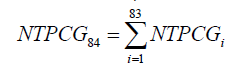
In this case, columns 86 and 87 are excluded from IOT quadrant II. Items 86-91 in column 72 are equal to the corresponding IOT items. To form line 72, a table of taxes and deductions (TTD) (Table 3) is introduced into the model, which is formed from n-vectors according to the number of taxes and deductions under consideration. In the proposed version of the model, as it was mentioned above, four types of taxes and deductions are considered. Each of the vectors consists of elements showing the amount of a particular tax or deductions for the corresponding economic sector. So, the elements of the first vector, marked as NTPCG, are determined by the amount of net taxes on products for consumer goods. For example, the element NTPCG14 is equal to the amount of net taxes on products used in the production of cellulose and paper (ES “Production of pulp, paper and paper products”, number 14 in the IOT). The elements of the NTPCG vector in the basic version are formed from the elements of line 86 of IOT (marked as IOT86) according to the following system of formulas (2):
NTPCGi=IO86i , for i = 1, 2, ..., 71, 73, ..., 83.85;
NTPCGi=IO86i+2 , for i = 86, 87, 88, 89;
NTPCG72=IO8672+IO8686+IO8687, for i = ; (2)
NTPCGi=IO86i , for i = ...
In the planning process, the elements of this vector are determined based on the assumption of proportionality of their change to the change in costs for the consumer products. The second vector, marked as CSSPF (Table 3), whose elements are equal to the contributions to the State Social Protection Fund of the corresponding economic sectors, in the basic version is compiled according to the data provided by the Belarus Agency for Official Statistics – Belstat. In the planning process, it is determined based on the expected salary for each economic sector and the percentage of deductions to the State Social Protection Fund.
| Table 3 Table of Taxes and Deductions (TTD) (Reference Year – 2017) |
||||||
|---|---|---|---|---|---|---|
| Line number | ES | |||||
| Crop and livestock production, provision of services in these sectors | … | State governing | … | Provision of other individual services | ||
| А | Б | 1 | … | 72 | … | 83 |
| Net taxes on products for consumer goods (NTPCG) | 1 | -527 277 | … | 113 286 | … | 9 986 |
| Other taxes on production (OTP) | 2 | 39 773 | … | 2 574 | … | 3 348 |
| Contributions to the State Social Protection Fund (CSSPF) | 3 | 626 719 | … | 730 999 | … | 40 676 |
| Income tax (IT) | 4 | 635 584 | … | 4 | … | 16 646 |
| Table 3.1 Table of Taxes and Deductions (TTD) (REFERENCE YEAR – 2017) |
|||||||
|---|---|---|---|---|---|---|---|
| Line number | Inter-mediate demand (sum of columns 01-83) | Final consumption expenditure | Gross fixed capital formation | Change in inventories | Export of goods and services | ||
| households | non-profit organizations providing services for households | ||||||
| А | B | 84 | 85 | 86 | 87 | 88 | 89 |
| Net taxes on products for consumed goods (NTPCG) | 1 | 3 991 660 | 6 047 148 | 1 471 | 405 173 | 70 568 | 3 491 378 |
| Other taxes on production (OTP) | 2 | 2 391 182 | 0 | 0 | 0 | 0 | 0 |
| Contributions to the State Social Protection Fund (CSSPF) | 3 | 11 004 100 | 0 | 0 | 0 | 0 | 0 |
| Income tax (IT) | 4 | 5 202 959 | 0 | 0 | 0 | 0 | 0 |
The third vector designated as IT and determining amount and rate of income taxes from an economic sector, is formed on the basis of the elements of line 92 of the IOT table and is calculated according to the assumed amounts of profit and income tax rates. The fourth vector of OTP, which determines other taxes on production in an economic sector, is formed from the elements of line 89 of the IOT table. Each of the last three vectors has 83 elements. The TTD obtained from these vectors, presented in Table 3, has 89 × 4 dimensions. TTD provides basic information for the calibration of the model in terms of taxes and deductions, which is carried out according to the reference year of 2017. This table will potentially provide information on the planned amounts of taxes and deductions. To implement this, we define the vector of TATD (total amount of taxes and deductions), which is the sum of the vectors that form the TTD (3):
TATD= NTPCG+CSSPF+IT+OTP (3)
In this case the elements of line 72 of the modified IOC table of the MIOT model (Table 4) are formed according to the formulas (4) - (5):
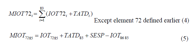
Element 85 in line 72 is equal to the state’s expenditure on social protection (SESP), which includes the expenditures on pensions and household payments from the State Social Protection Fund, excluding net taxes on products paid from households to the government. The basic value of these costs is, according to Belstat, 13,544,000 thousand rubbles. The model obtained in this way determines the amount of the total costs (according to the Leontief model) of each economic sector for the considered taxes and deductions per unit of the final product, depending on the volume of the final product of each economic sector and depending on the change in tax rates of any economic sector. Due to this, when planning changes in taxes and deductions of any economic sector, it is possible to determine how much the cost of products of each ES may change, including the cost of products of the ES itself, in which there have been changes in taxes and deductions. At that, it should be taken into account that if taxes on products for consumer goods, income tax and deductions to the SSPF can be considered as variable costs in case of no technological changes, then other taxes on production refer to constant ones. In this regard, two directions of modeling are considered:
• A model for static analysis, in which it is considered that the ES “State” provides services paid for by all four types of taxes and deductions presented in IOT in Table 3.
• A model for dynamic analysis, which uses the results of changes in production volumes of various economic sectors. In this case, taxes on products, income tax and deductions to the State Social Protection Fund are considered.
• The differences between these models are the following: the IOT in the first version includes four lines (table 3), in the second one – only the first three lines, accordingly, the vector of taxes and deductions (formula 3) changes in the following way:
TATD= NTPCG+CSSPF+IT (6)
Further we will consider the application of the developed model on the example of the ES 17 “Production of chemical products”. The reason for this choice is the potentially important role of this economic sector in the development of the national economy, the relative share of which in the manufacturing industry, represented in the IOT by twenty one ESs, is one tenth of its gross output. At that, the ES 17 “Production of chemical products” has quite stable relationships with the majority of ESs of the national economy, which justifies the selection of this ES as a demonstration example when testing the developed model of tax flows and deductions. The first option will be presented. The calibrated value of the amount of current taxes and deductions paid by the ES is 22,589,901 thousand rubles.
Analysis of changes in total costs by type of economic activity in case of change in the tax rate for the selected type of economic activity within the framework of the model for static analysis.
The importance of calculating the total costs of foreign economic activity for taxes and deductions is demonstrated by a comparison of direct and total costs for the considered taxes and deductions received from the ES 17 “Production of chemical products:
• For 1,000 rubles of the manufactured product, direct costs of taxes and deductions are 135.5 rubles;
• For 1,000 rubles of the final product, the total costs of taxes and deductions are 334.30 rubles.
Further, an economic policy scenario is considered, which involves stimulating the development of the ES 17 by reducing the income tax rate from 18% to 5%, and an assessment of the change in total costs for this case is also carried out. Taking into account the circumstances mentioned above, we will consider the change in total costs when the income tax rate for the ES 17 is reduced from 18% to 5%. This decrease in the rate leads to a decrease in income tax from 377,271 thousand rubbles to 104 797 thousand rubbles, i.e. by 272 473 thousand rubbles. If other conditions and parameters are equal, this means that the state will receive less of this amount as payment for its services and therefore this will lead to a decrease in intermediate demand (line 72 column 84) and, consequently, to a decrease in the total amount of money received by the state for its services from 26,080 142 thousand rubbles to 25 807 669 thousand rubbles. At the same time, according to Table 1, the difference between the amount of taxes and deductions received by the state and its expenses for its activities, called the “Conditional surplus of state’s activities”, also decreases by 272,473 thousand rubles, and, consequently, the volume of services provided by the ES 72 decreases as well. Next, we will consider the option assuming that the profit of the ES 17, which remains at its disposal, increases by the amount of the reduction in income tax, that is, by 272,473 thousand rubles. At the same time, the issue in monetary terms remains the same. The matrix of direct costs gives the following total indicators for all ESs, presented in Table 4.
| Table 4 Matrix of Direct Costs |
||||||
|---|---|---|---|---|---|---|
| ES number | AX | X | Y = X–AX | AX–AX caliber | X–X caliber | Y–Y caliber |
| 1 | 15 196 478 | 18 368 199 | 3 171 721 | 0 | 0 | 0 |
| 10 | 8 758 065 | 23 301 098 | 14 543 033 | 0 | 0 | 0 |
| 16 | 5 963 697 | 13 463 488 | 7 499 791 | 0 | 0 | 0 |
| 17 | 6 049 337 | 8 385 925 | 2 336 588 | 0 | 0 | 0 |
| … | … | … | … | 0 | 0 | 0 |
| 72 | 25 807 669 | 34 000 438 | 8 192 769 | -272 473 | -272 473 | 0 |
| 73 | 4 840 897 | 5 647 238 | 806 341 | 0 | 0 | 0 |
| 74 | 4 278 917 | 5 212670 | 753 | 0 | 0 | 0 |
| … | … | … | … | 0 | 0 | 0 |
| Sum | 141 430 314 | 236 330 618 | 94 900 304 | |||
From the information presented in Table 4, it can be seen that the final product (Y) remained the same as in the reference case, since the intermediate consumption of the ES 72 decreased due to the decrease in the tax on profits of the ES 17. In its turn, the output of the ES 72 in monetary terms decreased due to a decrease in profit, which, as expected, does not change the total value of the output of the final product of the ES 72. For a more complete analysis of the effect of the proposed changes, we present the matrices of total costs B-caliber and B and compare them. To illustrate, let us present an abbreviated version of the above matrices with the presentation for the analysis of individual foreign economic activities (Tables 5-6).
| Table 5 Matrix of Total Costs В-Caliber (Short), Thousand Rubles |
|||||||
|---|---|---|---|---|---|---|---|
| ES number | ES number | ||||||
| 1 | 10 | 16 | 17 | 72 | 73 | 74 | |
| 1 | 5 126 950 | 10 211 050 | 137 927 | 60 549 | 474 594 | 90 619 | 101 865 |
| 10 | 431 752 | 18 851 746 | 187 497 | 70 285 | 685 090 | 160 970 | 164 536 |
| 16 | 255 239 | 768 944 | 7 996 292 | 152 606 | 175 924 | 19 067 | 26 630 |
| 17 | 351 618 | 1 267 140 | 213 414 | 2 922 996 | 139 600 | 16 167 | 37 508 |
| 72 | 509 075 | 3 348 607 | 2 762 215 | 781 122 | 10 671 402 | 225 817 | 254 454 |
| 73 | 71 941 | 474 032 | 390 103 | 110 232 | 1 497 869 | 838 126 | 36 022 |
| 74 | 63 989 | 420 184 | 343 028 | 97 744 | 1 318 869 | 28 000 | 965 444 |
| Table 6 Matrix of Total Costs В (Short), Thousand Rubles |
|||||||
|---|---|---|---|---|---|---|---|
| ES number | ES number | ||||||
| 1 | 10 | 16 | 17 | 72 | 73 | 74 | |
| 1 | 5 126 519 | 10 210 198 | 138 806 | 55 356 | 479 292 | 90 693 | 101 912 |
| 10 | 431 129 | 18 850 518 | 188 766 | 62 789 | 691 871 | 161 077 | 164 604 |
| 16 | 255 079 | 768 629 | 7 996 618 | 150 681 | 177 665 | 19 094 | 26 648 |
| 17 | 351 491 | 1 266 890 | 213 673 | 2 921 469 | 140 981 | 16 189 | 37 521 |
| 72 | 495 401 | 3 302 998 | 2 759 864 | 659 078 | 10 691 357 | 225 679 | 253 480 |
| 73 | 70 579 | 471 345 | 392 877 | 93 843 | 1 512 696 | 838 360 | 36 170 |
| 74 | 62 789 | 417 819 | 345 471 | 83 314 | 1 331 924 | 28 207 | 965 575 |
Comparison of the matrices of total costs B and B-caliber produces the values of the indicators presented in Table 7 (an illustrative short version of the matrix B caliber – B is presented).
| Table 7 Matrix of Total Costs B – В-Caliber (Short) |
||||||||
|---|---|---|---|---|---|---|---|---|
| ES number | Sum for all ESs | |||||||
| 1 | 10 | 16 | 17 | 72 | 73 | 74 | ||
| 1 | 432 | 851 | -879 | 5 193 | -4 698 | -74 | -47 | 0 |
| 10 | 623 | 1 229 | -1 269 | 7 496 | -6 782 | -107 | -68 | 0 |
| 16 | 160 | 316 | -326 | 1 925 | -1 741 | -28 | -17 | 0 |
| 17 | 127 | 250 | -259 | 1 527 | -1 382 | -22 | -14 | 0 |
| 72 | 13 675 | 45 609 | 2 352 | 122 044 | -19 955 | 138 | 973 | 272 473 |
| 73 | 1 362 | 2 686 | -2 774 | 16 389 | -14 827 | -234 | -148 | 0 |
| 74 | 1 199 | 2 365 | -2 443 | 14 431 | -13 055 | -206 | -131 | 0 |
| Sum | 17 578 | 53 307 | -5 598 | 169 005 | -62 439 | -534 | 548 | – |
From the matrix presented in Table 7, it can be seen that, despite the unchanged volumes of total costs of products of each ES, the distribution of total costs between the ESs has changed. Thus, the presented calculations showed that a change in tax rates, even with unchanged volumes of the final product, leads to a redistribution of total costs between ESs. It should also be noted that the distribution between ESs of the full costs of taxes and deductions, as can be seen from Table 8, is more even than the distribution of direct costs. This is confirmed by calculations of the relative standard deviation: direct costs 55%, total – 23%, respectively (the calculations did not take into account government costs).
| Table 8 Share of Direct and Total Costs of Taxes and Deductions in the total Amount of the Corresponding Costs for a ES |
|||||||||||||||||
|---|---|---|---|---|---|---|---|---|---|---|---|---|---|---|---|---|---|
| Name of value | ES number | ||||||||||||||||
| 1 | 2 | 3 | 4 | 5 | 6 | 7 | 8 | 9 | 10 | 11 | 12 | 13 | 14 | 15 | 16 | 17 | |
| Shdir3 | 4 | 37 | 27 | 22 | 0 | 38 | 0 | 24 | 38 | 8 | 18 | 18 | 16 | 11 | 15 | 8 | 22 |
| Shtot | 6 | 14 | 13 | 10 | 0 | 16 | 0 | 13 | 15 | 8 | 12 | 12 | 12 | 10 | 11 | 12 | 13 |
| Name of value | ES number | ||||||||||||||||
| 18 | 19 | 20 | 21 | 22 | 23 | 24 | 25 | 26 | 27 | 28 | 29 | 30 | 31 | 32 | 33 | 34 | |
| Shdir3 | 28 | 12 | 17 | 9 | 14 | 19 | 13 | 16 | 16 | 6 | 16 | 16 | 21 | 12 | 72 | 14 | 24 |
| Shtot | 14 | 11 | 12 | 10 | 11 | 12 | 11 | 11 | 11 | 8 | 11 | 12 | 12 | 12 | 20 | 12 | 13 |
| Name of value | ES number | ||||||||||||||||
| 35 | 36 | 37 | 38 | 39 | 40 | 41 | 42 | 43 | 44 | 45 | 46 | 47 | 48 | 49 | 50 | 51 | |
| Shdir3 | 27 | 16 | 19 | 17 | 34 | 25 | 23 | 26 | 34 | 10 | 20 | 52 | 28 | 18 | 25 | 21 | 20 |
| Shtot | 13 | 11 | 12 | 11 | 14 | 13 | 12 | 13 | 15 | 11 | 10 | 18 | 13 | 10 | 12 | 12 | 12 |
| Name of value | ES number | ||||||||||||||||
| 52 | 53 | 54 | 55 | 56 | 57 | 58 | 59 | 60 | 61 | 62 | 63 | 64 | 65 | 66 | 67 | 68 | |
| Shdir3 | 21 | 68 | 35 | 43 | 67 | 46 | 30 | 55 | 42 | 47 | 33 | 22 | 48 | 54 | 37 | 33 | 21 |
| Shtot | 12 | 17 | 14 | 14 | 17 | 15 | 12 | 16 | 15 | 15 | 14 | 12 | 15 | 16 | 13 | 13 | 12 |
| Name of value | ES number | ||||||||||||||||
| 69 | 70 | 71 | 73 | 74 | 75 | 76 | 77 | 78 | 79 | 80 | 81 | 82 | 83 | ||||
| Shdir3 | 26 | 29 | 26 | 46 | 32 | 35 | 27 | 39 | 38 | 21 | 34 | 27 | 34 | 32 | |||
| Shtot | 13 | 13 | 12 | 14 | 13 | 13 | 12 | 14 | 14 | 12 | 14 | 13 | 13 | 14 | |||
Explanation: Shdir3 – the share of direct costs for taxes and deductions in the total amount of all direct costs; Shtot – the share of the total cost of taxes and deductions in the total amount of all total costs.
The information presented as a result of the calculations based on the developed model should be taken into account when assessing the impact of reducing the tax burden for a specific ES on reducing its costs, taking into account the influence of the tax burden on suppliers of an ES, which smooths out the positive effect of a direct reduction in the tax burden for a specific foreign economic activity. We should also mention that the quantitative assessment of the results of the described mutual influence is possible only by using the presented model of tax flows and deductions in planning the development of the national economy. Next, let us consider a scenario in which the development of the national economy required the ES 17 to increase the production of the final product by 20%.
Analysis of changes in total costs by type of economic activity when the volume of final products in the selected ES changes in the framework of the model for dynamic analysis
Analysis of the change in the total costs of an ES when the tax rate for the selected ES changes within the framework of the model for dynamic analysis, as noted above, assumes the exclusion of other taxes on production from this analysis. Compared to the previous case, other taxes on production are included in quadrant III of the model. In the general case, when any taxes and deductions are excluded from the analysis, they are removed from the IOT and transferred to the third quadrant of the model. The calibrated value of the amount of the analyzed taxes is equal to 20 198 712 thousand rubles. Perspectively, we are talking only about net taxes on products for used goods, income tax and contributions to the State Social Protection Fund. The calculation of the “Conditional surplus of state’s activities” is done similarly to the previous version, taking into account the change in the volume of the ES 72, since services paid for by other taxes on production are excluded from there. The calculated value of the indicator “Conditional surplus of state’s activities” is presented in Table 9.
| Table 9.1 Calculating Value for the Indicator “Conditional Surplus of State’s Activity”, Variant 2 |
|||||||
|---|---|---|---|---|---|---|---|
| А | Line number | ES | Inter-mediate demand (sum of columns 01-83) | Final consumption expenditure on | |||
| … | State admini-stration and governance | … | households | non-profit organizations providing services for households | |||
| Б | 1-71 | 72 | 73-83 | 84 | 85 | 86 | |
| … | 1-71 | … | |||||
| State governing and defense services provided to society; compulsory social insurance services | 72 | … | … | 24 478 592 | 8 162 220 | ||
| Table 9.2 Calculating Value for the Indicator “Conditional Surplus of State’s Activity”, Variant 2 |
|||||
|---|---|---|---|---|---|
| Gross fixed capital formation | Change in inventories | Export of goods and services | Total amount of resources of goods and services consumed at basic prices (sum of columns 84-89) | Import of goods and services … | Total amount of domestic goods and services consumed at basic prices (columns 90- 91) |
| 87 | 88 | 89 | Б | 1-71 | 72 |
| 42 258 | 32 683 070 | 11 709 | 32 671 361 | ||
| Table 9.3 Calculating Value for The Indicator “Conditional Surplus of State’s Activity”, Variant 2 |
|||
|---|---|---|---|
| Total used in customer prices (sum of lines 01-85) | 86 | … | 18 531 909 |
| Salary (remuneration of labor without contributions to the State Social Protection Fund) | 87 | … | 2 568 356 |
| Other taxes on production | 88 | … | 2 574 |
| Fixed capital consumption | 89 | … | 425 582 |
| Profit exclusive of income tax (conditional surplus of state’s activity) | 90 | … | 11142 939* |
| Production of goods and services at basic prices (sum of lines 86-80) | 91 | … | 32 671 361 |
At this stage we will consider the growth of production volumes of the final product of the ES 17 “Chemical production” by 20%. Increasing the seventeenth element of the vector of the final product Y in the model under consideration by 20%, i.e., from 2,336,588 thousand rubles to 2 803 906 thousand rubles, we get the following changes in production volumes X of each of the ESs presented in Table 10.
| Table 10 Changes in production volumes (x) of individual foreign economic activities with an increase of 20% in production volumes of the final product (y) of the ES 17 “chemical production” |
||||
|---|---|---|---|---|
| ES number | Production volume (Х), mln roubles | Change (+, –) | ||
| X new | X reference | Absolute | Relative, % | |
| 1 | 18 379 253 | 18 368 199 | 11 054 | 0,06 |
| … | … | … | … | … |
| 7 | 0 | 0 | 0 | 0,00 |
| 8 | 465 972 | 453 643 | 12 329 | 2,72 |
| 9 | 37 678 | 34 397 | 3 281 | 9,54 |
| 10 | 23 313 631 | 23 301 098 | 12 533 | 0,05 |
| 11 | 3 051 352 | 3 048 016 | 3 336 | 0,11 |
| 12 | 720 121 | 719 643 | 478 | 0,07 |
| 13 | 2 712 859 | 2 711 349 | 1 510 | 0,06 |
| 14 | 981 246 | 976 649 | 4 597 | 0,47 |
| 15 | 386 530 | 385 774 | 756 | 0,20 |
| 16 | 13 493 618 | 13 463 488 | 30 130 | 0,22 |
| 17 | 8 970 214 | 8 385 925 | 584 289 | 6,97 |
| 18 | 1 143 619 | 1 141 632 | 1 987 | 0,17 |
| … | … | … | … | … |
| 72 | 22 046 250 | 21 919 949 | 126 301 | 0,58 |
As can be seen from the information presented in Table 10, the increase in the final product of the ES 17 by 467,318 thousand rubles requires an increase in the production of this ES by 584,289 thousand rubles, i.e. by 7%. At the same time, the total costs of the ES 17 for products of each ES increase by 20% (Table 11).
| Table 11 Total Costs of The Es 17 – Reference and Prognosed Values |
|||
|---|---|---|---|
| Total costs of the ES 17, troubles | Increase in total costs, % | ||
| Reference | New | ||
| Total | 5622 186 | 6 746 623 | 20 |
| For taxes and deduction | 631 502 | 757 803 | 20 |
Table 11 shows that the increase in total costs is proportional to the increase in the volume of the final product, which follows from the formula for calculating the total costs (TC):
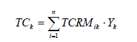
Where TCRM is the total cost ratio matrix;
TCk – The amount of the total costs of the element k of the vector Y;
n – The number of ESs.
If the argument Yk is multiplied by any number, then, as follows from the linearity of the given formula in Y, the value of ПЗk will also be multiplied by this number. Due to the increase in tax payments, the total costs of the ES 17 will increase by 126,301 thousand rubles (757 803 – 631 502). Direct costs of taxes will increase in proportion to the increase in the volume of production of this ES, i.e., by 7%, which in absolute terms will amount to 67,948 thousand rubles (970,681 × 7%). Consequently, due to an increase in the output of the final product of the ES 17 by 20%, the state will receive an additional 126,301 thousand rubles of taxes and deductions. At the same time, 46% of this amount will be received by the state from other ESs.
Taking into account the abovementioned, it can be concluded that the model of tax flows and deductions presented in the article allows determination of direct and total costs and their structure for tax payments and deductions of any economic sector, calculation changes in total and direct costs of taxes and deductions that can be attributed to variable costs when the volume of production of the final product changes, and determination of the full amount and structure of the increase in taxes and deductions to the state/ The model also allows to analyze changes in the total and direct costs of paying taxes and deductions at different tax rates for the selected ES, as well as to solve other problems within the framework of the state tax policy arising from forecasting and planning at the level of interaction between ESs, i.e., at the level that connects macroeconomic and sectoral planning. The need to solve the above problems arises when analysing the mutual influence of ESs on the taxes and deductions paid by them in forecasting and planning at the level of interaction between ESs, i.e., at the level that connects macroeconomic and sectoral planning.
References
ASM. (1960). A social accounting matrix. Stone, London: Chapma, Hall.
Crossref , Google scholar , Indexed at
Brown, D.K. (2001). CGE modeling and analysis of multilateral and regional negotiating options. Research Seminar in Intern. Economics, University of Michigan: School of Public Policy.
Khan, H.A. (2007). Social Accounting Matrices (SAMs) and CGE modelling: using macroeconomic computable general equilibrium models for assessing poverty impact of structural adjustment policies.
Korotkevich, A.I. (2017). Synthetic model of the national economic system of the Republic of Belarus based on modified input-output tables.
Korotkevich, A.I. (2019). Improvement of forecasting, planning and analysis tools for the development of the national economic system of Belarus: monograph.
Crossref , Google scholar , Indexed at
Korotkevich, A.I. (2017). Modeling of the national economic system of Belarus and the direction of its transformation.
Crossref , Google scholar , Indexed at
Leontief, W.W. (2007). Selected works: in 3 volumes/W.W. Leontief–M: Economics, 2006-2007.
McKitrick, R.R. (1998). The econometric critique of computable general equilibrium modeling: the role of functional forms.Economic Modelling, 15(4), 543-573.
Crossref , Google scholar , Indexed at
Pyatt, G. (1979). Accounting and fixed price multipliers in a social accounting matrix framework.The Economic Journal, 89(356), 850-873.
Crossref , Google scholar , Indexed at
Shparun, D.V. (2017). Method of planning tax collections. Belarusian Economic Journal, 2, 53-66.
System of tables “Input – Output” of the Republic of Belarus for 2017: stat. bul. // National Statistical Committee of the Republic of Belarus – Minsk,
Zakharchenko, N.G. (2012). Using matrices of state budget accounts in modeling the structure of an economic system. Spatial Economics, 1, 69-89.
Received: 27-Dec-2021, Manuscript No. ASMJ-21-9042; Editor assigned: 29-Dec-2021, PreQC No. ASMJ-21-9042(PQ); Reviewed: 10-Jan-2022, QC No. ASMJ-21-9042; Revised: 20-Jan-2022, Manuscript No. ASMJ-21-9042(R); Published: 27-Jan-2022