Research Article: 2019 Vol: 18 Issue: 4
Strategic Handout of Economic Sides to Economic Extension in Bangladesh: An ARDL Bound Test Approach
Shanjida Chowdhury, Daffodil International University
Afrina Akter Mishu, Comilla University
Nasir Uddin, Daffodil International University
Sara Tasneem, Dhaka School of Economics
Nurul Mohammad Zayed, Daffodil International University
Abstract
Keywords
Contribution, Economic Growth, Agriculture, Manufacturing, Service, Bangladesh.
JEL Classifications
010.
Introduction
The economic health of any nation is prognoses through the contribution of the sectorsagriculture, manufacturing, and service. The highest ever growth achieved considering the new base year of 2005-06 for estimating national accounts in Bangladesh. Contribution of agricultural sector is around 14.23% in 2017-18 fiscal years but once it was around 40 percent after independence and 16% in 2014-15 fiscal years. One sharp observation is in manufacturing, 20% from 2014-15 is now 22.85% (BBS, 2018). As the economy is changing, the proportion of manufacturing is also shifting. According to the Bangladesh Bureau of Statistics (BBS), the contribution of the manufacturing sector is the highest in Gross Domestic Product (GDP). It is the basis of GDP for any developing societies, is almost half of its total. This study examines the contributions of Agriculture (AGR), Manufacturing (MAN) and Services (SER) sector on annual growth of GDP of Bangladesh. Also, this study tries to grasp the direction of short run and long run towards economic growth.
Literature Review
Ahmad et al. (2016) examined a relationship in Pakistan for the period from 1989 to 2012 and study found that GDP of Pakistan will be positively influenced due to growth in agricultural and manufacturing sectors. Rahman et al. (2011) scrutinized Granger causality in their study and long run equilibrium relationship also found in this study. Azer et al. (2016) after using correlational and multiple regression analysis on the time series data for the year 2000 until 2010, suggested that manufacturing and service sectors are significantly related to GDP per capita in Malaysia. Gaspar et al. (2015) used co-integration and causality data analysis techniques for investigating the links between agriculture and non-agricultural sectors in Portugal for the period 1970-2006.The study found that in Portugal, agriculture has no influence on the expansion of service and industry sector in the long-run. On the other hand, agriculture also receives no influence from the growth in other sectors. Uddin (2015) found unidirectional Granger causality in Bangladesh by examining industry, service sector and agricultural contribution to Bangladesh economy. The study follows this paper but using updated data. Because over time period sectoral contribution also changes as the size of Bangladesh economy is becoming larger and more diversified. Sectorial factors-agriculture, manufacturing, and service are accounted for this study from 1990 to 2017. Also; it tries to grasp the direction of short run and long run towards economic growth. For this, the ARDL method is implicated.
Methodology
This study used an annual time series data covering the period from 1990 to 2017 of Bangladesh. The data were retrieved from the online version of World Development Indicators (WDI), the World Bank database. The variables are measured in millions, US$ dollar in current price. Secondary data is appropriate here, as this study scrutinizes the contributions of AGR, MAN and SER sector on annual growth of GDP of Bangladesh. After unit root test, we examine the long-run relationship among gross domestic product (LNGDP), agriculture (LNAGR), manufacture (LNMAN) and service (LNSER). We employed ARDL bound test to analyze where there is a long run relationship or not. Hence, the ARDL model is:
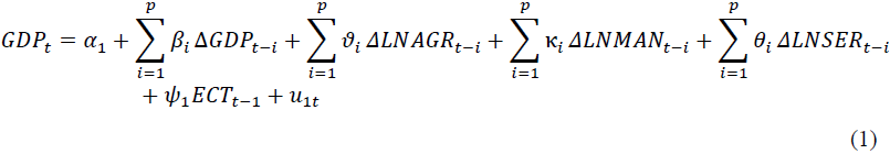
The ARDL bound test tells us that if F-value surpasses the tabulated value at 5% level of significance, then there is a co-integration of study variables. On the model, it is significant also for 1 percent level of significance, so it can be conclude that there is a strong relationship of economic growth and defense spending.
Results and Discussion
In the study, we employ both Augmented Dickey-Fuller (ADF) test (Dickey & Fuller, 1979: 1981) & PP (Phillips-Perron) test for 4 variables (Table 1). To solve hetero-scedasticity, we consider natural log form of all variables. Though service (LNSER) reveals stationary in the ADF test, it doesn’t stationary at the level in PP test. Hence, all are stationary at first difference that is, all variables are I (1) series. ARDL bound testing approach to long run level relationship among the variables requires the determination of the optimal lag for the co integrating equation based on the assumption of serially uncorrelated residual.
| Table 1 Unit Root Test | ||||||
| ADF Test | PP Test | |||||
| Variable | Constant | Trend and Constant | Decision | Constant | Trend and Constant | Decision |
| LNGDP | 3.2258 | -0.6451 | Unit Root | 2.8263 | -0.6738 | Unit Root |
| D(LNGDP) | -3.1816** | -3.7645** | Stationary | -3.1191** | -3.6613** | Stationary |
| LNMAN | -1.5091 | -2.1456 | Unit Root | -1.5091 | -2.1456 | Unit Root |
| D(LNMAN) | -3.5888** | -3.8822** | Stationary | -4.4072*** | -4.3956*** | Stationary |
| LNSER | -14.4776*** | -6.6079*** | Stationary | -1.0694 | -2.0188 | Unit Root |
| D(LNSER) | -6.8966** | -7.964** | Stationary | -7.2668*** | -21.4443*** | Stationary |
| LNAGR | -0.4368 | -2.8182 | Unit Root | -0.1876 | -2.7328 | Unit Root |
| D(LNAGR) | -6.5883** | -6.5486** | Stationary | -7.0462*** | -7.8828*** | Stationary |
Source: Estimated.
The lag length that minimizes the value of the AIC, SC, HQ and SBC and at which the model does not have autocorrelation is the optimal lag. The Schwarz Information Criterion (SC) was used to select the optimal lag length (Table 2).
| Table 2 Lag Length Selection | ||||||
| Lag | LogL | LR | FPE | AIC | SC | HQ |
| 1 | 338.3115 | 176.8579 | 1.05E-16 | -25.4649 | -24.48982 | -25.1945 |
| 2 | 363.1589 | 31.80465 | 5.78e-17 | -26.17271 | -24.4175 | -25.68590 |
| 3 | 379.1312 | 15.3334 | 7.95E-17 | -26.1705 | -23.6352 | -25.4673 |
Table 3, discloses that we cannot take lag order more than 2 in case of annual data. The OLS employ with unrestricted regression. Maximum order as 3 for ARDL procedure is chosen for the required data set. The critical value that reported together in the same table was based on critical value suggested by (Narayan, 2004). Since our F-statistic is 20.05509 with degrees of freedom (3,24), which surpasses the upper bound critical value at 1% level of significance using unrestricted regression with constant. So it rejects the null hypothesis of having no co integration. So we can conclude that there is a strong co-integrating relationship among variables.
| Table 3 F-statistic of Co-integration Relationship | |||||
| Test Statistic | Value | Lag | Level of Significance | Bound Critical values(restricted Constant and no trend) | |
| F-Statistic | 20.05509 | 3 | I(0) | I(1) | |
| 10% | 2.72 | 3.77 | |||
| 5% | 3.23 | 4.35 | |||
| 2.50% | 3.69 | 4.89 | |||
| 1% | 4.29 | 5.61 | |||
The long-run model (Table 4) reveals significant using ARDL (1, 2, 0, and 2) model. Except for manufacturing (LNMAN), all are significant at 1% level of significance. That means GDP will decrease 6.13 units if agricultural input will increase 1 unit. Seemingly, GDP will decrease 13.66 units if input of service industry will increase 1 unit. So, in long run model, agriculture and service are converges with GDP but negative direction.
| Table 4 Long Run Co-efficient for ARDL (1, 2, 0, 2) Model | ||||
| Variable | Coefficient | Std. Error | t-Statistic | Prob. |
| LNAGRI | -6.132117 | 0.767748 | -7.987151 | 0 |
| LNMAN | -0.424507 | 0.878938 | -0.482978 | 0.6353 |
| LNSER | -13.66234 | 2.348452 | -5.817593 | 0 |
In case of short run for ARDL (1, 2, 0, and 2) model (Table 5), the coefficient of each variable at first difference is significant at 1% level of significance. Also, ECT, error correction mechanism term reveals significant short-run adjustment of GDP with respect to others In addition; the ECM term means GDP is converged to other variables to the long run equilibrium by 24.105% in one period with speed of adjustment. Also, each variable is a significant but positive relationship with GDP. But there’s an interesting view that the long run model reveals negative with study variables.
| Table 5 Short Run Coefficients for ARDL (1, 2, 0, 2) Model | ||||
| Variable | Coefficient | Std. Error | t-Statistic | P-value |
| C | 8.363361 | 0.85777 | 9.750119 | 0.0000 |
| D(LNAGRI) | 0.101729 | 0.270714 | 0.375779 | 0.7117 |
| D(LNAGRI(-1)) | 1.399771 | 0.302756 | 4.623435 | 0.0002 |
| D(LNSER) | 0.49277 | 0.419278 | 1.175282 | 0.2561 |
| D(LNSER(-1)) | 2.065365 | 0.490679 | 4.2092 | 0.0006 |
| ECT(-1) | -0.24105 | 0.024813 | -9.71478 | 0.0000 |
From Figure 1, both CUSUM and CUSUMSQ tests indicate that the ARDL model is steady and specified appropriately.

Figure 1 Stability Test (Cusum &Cusumsq Test)
Also, diagnostic test (Table 6) is employed for hetero-scedasticity, autocorrelation, model specification, and normality test.
| Table 6 Diagnostic Test | |||
| Heteroscedasticity Test: Breusch-Pagan-Godfrey | |||
| F-statistic | 0.792 | Prob. F(8,17) | 0.6172 |
| Obs*R-squared | 7.057 | Prob. Chi-Square(8) | 0.5305 |
| Heteroscedasticity Test: ARCH | |||
| F-statistic | 0.31 | Prob. F(1,23) | 0.5832 |
| Obs*R-squared | 0.332 | Prob. Chi-Square(1) | 0.5643 |
| Breusch-Godfrey Serial Correlation LM Test | |||
| F-statistic | 0.788 | Prob. F(2,15) | 0.4729 |
| Obs*R-squared | 2.471 | Prob. Chi-Square(2) | 0.2907 |
| Jarque-Bera Test | |||
| Test statistic | 1.500553 | ||
| Prob. | 0.472236 | ||
| Reset Test | |||
| Value | df | Probability | |
| t-statistics | 0.20296 | 16 | 0.8417 |
| p-value | 0.04119 | (1,16) | 0.8417 |
Conclusions and Policy Implications
This study adorned the ARDL model from 1990 to 2017 to revisit sectoral contribution on GDP. Yetiz & Özden (2017) and Uddin (2015) examine same work employing Johansen cointegration and Granger Causality. This study revealed the significant relationship in the short run of economic growth with three sectoral inputs. In the short run, ECM (Error Correction Mechanism) postulates that GDP is converged to control variables to the long run equilibrium by 24.105% in one period with speed of adjustment. In long run, manufacturing retards significant long-run relation with economic growth. But other sectoral variables display a significantly negative relationship with economic growth. Nevertheless, the study coincides some negative relationship of economic growth with explanatory variables. This study helps policymakers to reexamine their step for promoting the service sector more, but not lagged behind our agricultural feedback. Like as a developing country, Bangladesh stands on the basis of three pillar- agriculture, service, and manufacturing. Except one, other will be loose down and hamper our economic stability optimization. To snap about economic health, government, as well as private think tankers, should be updated with contemporary research. This paperwork also revisits and rethinks about the contribution of donors or government sides.
References
- Ahmad, Z., Iqbal, F., & Mehmood, S. (2016). Relationship between sectors shares and economic growth in Pakistan: A time series modeling approach. Journal of Statistics, 23(1).
- Azer, I., Hamzah, H.C., Mohamad, S.A., & Abdullah, H. (2016). Contribution of economic sectors to Malaysian GDP. In Regional Conference on Science, Technology and Social Sciences (RCSTSS 2014), Springer, Singapore, 183-189.
- BBS (2018). 2017 statistical year book of Bangladesh, Dhaka. Bangladesh Bureau of Statistics.
- Dickey, D.A., & Fuller, W.A. (1979). Distribution of the estimators for autoregressive time series with a unit root. Journal of the American Statistical Association, 74(366a), 427-431.
- Dickey, D.A., & Fuller, W.A. (1981). Likelihood ratio statistics for autoregressive time series with a unit root. Econometrica: Journal of the Econometric Society, 1057-1072.
- Gaspar, J., Gilson, P., Simoes, M.C.N. (2015). Agriculture in Portugal: Linkages with industry and services. Faculdade de Economica da Universidade de Coimbra.
- IMF (2018). Article IV consultation-press release; staff report; and statement by the executive director for Bangladesh. Washington, D.C.
- Narayan, P. (2004). Reformulating critical values for the bounds F-statistics approach to cointegration: An application to the tourism demand model for Fiji, 2(04). Australia: Monash University.
- Rahman, M.M., Rahman, M.S., & Hai-bing, W.U. (2011). Time series analysis of causal relationship among GDP, agricultural, industrial and service sector growth in Bangladesh. China-USA Business Review, 10(1), 9-15.
- Uddin, M.M.M. (2015). Causal relationship between agriculture, industry and services sector for GDP growth in Bangladesh: An econometric investigation. Journal of Poverty, Investment and Development, 8.
- Yetiz, F., & Özden, C. (2017). Analysis of causal relationship among gdp, agricultural, industrial and services sector growth in Turkey. Ömer Halisdemir University Journal of the Faculty of Economics and Administrative Sciences , 10(3), 75-84.